Blog/Best Practice

Kwai Vector Search on Paimon with Apache Doris

Apache Doris · Wenqiang Li; Kwai · Junrui Li, Shiyao Yu, Fangyuan DengSeptember 10, 2026

Introduction:

Kwai uses Apache Doris in production to query vector indexes directly on Apache Paimon tables. Vectors and business data remain in Paimon, while Doris SQL initiates retrieval and pushes execution down to the data lake. Existing ingestion pipelines and OLAP access patterns do not change. This article explains the indexing foundation in Paimon 2.0, the read path developed jointly by the Doris and Paimon communities, and benchmark results for tens of millions and hundreds of millions of vectors.

As LLM and RAG applications have become more common, semantic search has become a standard data platform requirement. One common design synchronizes vectors, filter fields, and result fields into a standalone vector database. The main cost is not the initial synchronization but the ongoing maintenance. Synchronization pipelines must run continuously, which creates a data freshness window. Vectors and business fields are split across two systems, as are access control and governance. Teams also need additional safeguards to maintain consistency between the systems.

Kwai took a different approach. Vectors and business columns remain in Paimon tables, and the Vector Index in Paimon 2.0 handles retrieval. Doris reads indexes and data directly through Paimon Rust. It retrieves candidates and looks up rows in parallel by bucket. Users continue to write Doris SQL with the same syntax they use for Doris internal tables.

Availability: Kwai has validated this integration in production, while the Doris 4.2 capabilities described here are scheduled for public release at the end of September.

1. Data foundation: indexing in Paimon 2.0

1.1 Physical separation of indexes and data

The Vector Index in Paimon 2.0 works with ordinary Paimon tables and has two forms: the Global Vector Index for append tables and the PK Vector Index for primary-key tables. Both use the same index implementation and retrieval model, but they build indexes and retrieve matching rows differently. Kwai's business tables are primary-key tables, so the rest of this article focuses on the PK Vector Index.

Both forms store index files separately from data files. A Snapshot references a Data Manifest and an Index Manifest. The Index Manifest records each index file's type, field, location, and coverage. For append tables, it records the covered Row ID range. For primary-key tables, it records the covered source data files. Adding an index therefore does not require a different data layout, and the same table can still support batch processing, stream processing, and regular OLAP reads.

Figure 1 shows how index files relate to data files.

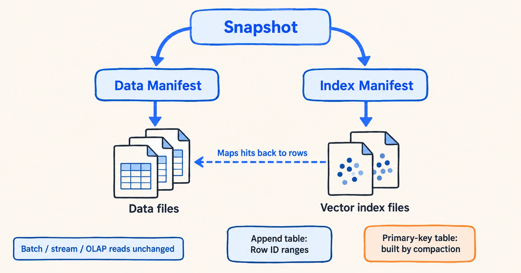
Figure 1: Index files and data files are stored separately. The same Snapshot links them through two types of Manifest. Index segments for primary-key tables are generated during compaction and record their source files.

Vector columns are declared as ARRAY<FLOAT> or fixed-length VECTOR<FLOAT, N>. For primary-key tables, table properties configure vector indexes, which are built automatically during compaction without a separate trigger. The following Spark SQL specifies the indexed column, index type, and distance metric when creating a primary-key table:

CREATE TABLE vector_items (
item_id BIGINT,
embedding ARRAY<FLOAT> COMMENT '__VECTOR_FIELD;2048',
payload STRING
) TBLPROPERTIES (
'primary-key' = 'item_id',
'bucket' = '32',
'deletion-vectors.enabled' = 'true',
'pk-vector.index.columns' = 'embedding',
'fields.embedding.pk-vector.index.type' = 'ivf-rq',
'fields.embedding.pk-vector.distance.metric' = 'l2'
);

• Spark SQL does not have a VECTOR type. The column comment __VECTOR_FIELD;2048 declares ARRAY<FLOAT> as a fixed-length, 2,048-dimensional vector.
• Build parameters such as nlist are passed as JSON through fields.<col>.pk-vector.index.options.
• The reranking multiplier refine_factor can be set in either table properties or query options.

After data is written, compaction merges files within a bucket into a level above Level 0 and generates an index segment for the vector column. A new Snapshot references the segment after it is registered in the Index Manifest. The segment records the source data files it covers, which allows matches to map back to physical row positions within those files. Newly written data does not belong to an index segment until the next compaction. Section 2.2 explains how retrieval handles this intermediate state.

1.2 Five types of vector indexes

The Paimon 2.0 Vector Index currently supports five index implementations, each with different characteristics and trade-offs:

Index	Main characteristic	Typical trade-off
IVF-Flat	Stores the original vectors after clustering	Higher recall, but a larger index
IVF-PQ	Product quantization	Smaller index, but some quantization loss
IVF-SQ	8-bit scalar quantization of residuals	Balanced throughput, recall, and storage
IVF-RQ	Rotated residual quantization	Higher compression, but requires tuning around the quality inflection point
DiskANN	Graph search with persistently stored vectors for reranking	Suitable for local SSDs or a fully local cache

The index types balance query performance, recall, index size, and build time differently. Storing hundreds of millions of 2,048-dimensional vectors at their original precision produces a correspondingly large index and increases the amount of data read from remote storage. RQ uses rotated residual quantization to achieve greater compression, though it must be tuned to meet quality targets. Kwai chose IVF-RQ as a balance between compression and recall. The measured Recall in Section 3.3 ranges from 96.0% to 99.6%.

Figure 2 compares the five index types and shows Kwai's choice.

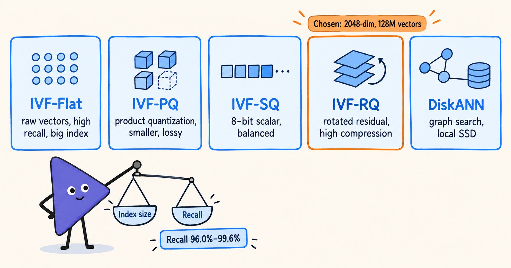
Figure 2: Each index type makes a different trade-off between index size and recall. Kwai chose IVF-RQ and used its higher compression to reduce remote reads.

2. Bringing indexes back to the data lake: how Doris directly queries Paimon indexes

A compute engine needs the following capabilities to use indexes on lake data directly for retrieval:

• A high-performance data read path.
• Awareness of index distribution and index coverage.
• Optimized index access for common vector-retrieval workloads such as Top-K.

Together, these capabilities allow the engine to retrieve and analyze lake data efficiently. Section 2.1 covers the read path. Section 2.2 explains index awareness and retrieval pushdown. Sections 2.3 and 2.4 describe two index-access optimizations for Top-K workloads.

2.1 High-performance reads: from JNI to Paimon Rust

In earlier Doris versions, reading Paimon data in MOR (Merge-On-Read) scenarios required the Paimon Java SDK. Doris called the SDK through JNI to read and merge the data. This approach had two problems:

• Doris could not track and control JVM memory at query granularity. If a large query exhausted memory, Doris lacked fine-grained visibility and control over its usage.
• MOR used substantial memory, and high concurrency could cause JVM OOM errors. Increasing the JVM heap reduced the native memory available to the BE.

After testing both options, Kwai chose Paimon Rust. The official Paimon team maintains Paimon Rust and keeps its MOR and index reads in sync with the Java implementation. Tests found that Paimon Rust provided two to three times the read performance of Paimon Java and was approximately 10% slower than the native Doris reader. Most of the difference came from converting Arrow's in-memory format into Doris Blocks. Paimon Rust uses native memory, so Doris can include its consumption in the existing memory-control system and manage it together with other native memory.

At the code level, the Doris BE, which is the C++ execution process, calls the Paimon Rust Reader through a C ABI. Rust and C++ exchange results through the Arrow C Data Interface. Doris then converts those results into Doris Blocks and passes them to the execution layer. Because Arrow is a columnar format, C++ can consume the data produced by Rust directly by column without an intermediate row-by-row conversion.

Figure 3 shows this read path.

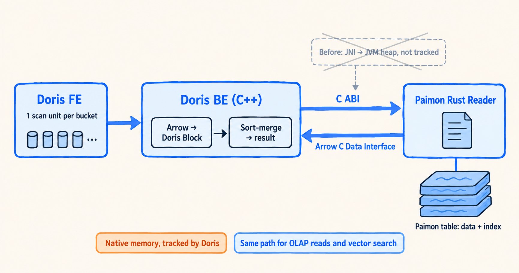
Figure 3: Doris BE calls Paimon Rust through a C ABI. Paimon Rust returns results in Arrow's columnar format, which Doris converts into Blocks. Regular reads and vector retrieval use the same path.

2.2 Pushing retrieval down to the data lake

Unlike a regular read, a vector Top-K query does not know which rows it needs before reading starts. It must identify those rows through the index first. Without the index, a vector Top-K query written as ORDER BY ... LIMIT becomes a full computation. Doris loads the entire vector column into BE memory, calculates distances row by row, and sorts the results. For 128 million rows with 2,048 dimensions, one query would need to transfer approximately 1 TB of vector data.

The query engine must push retrieval down to the index on the data lake. To do this correctly, it must account for four properties of vector indexes on Paimon primary-key tables:

• Indexes are organized by (Partition, Bucket). A bucket is both the data-sharding unit and the indexing unit.
• Paimon's background compaction process generates indexes, so indexes cover only compacted data. Newly written L0 files are not included in any index. Correct retrieval must merge three operations: index retrieval, exact fallback over uncovered files, and Deletion Vector mask computation.
• An index segment is valid only when its set of covered source files still matches the bucket's current set of active files. Checking this condition requires the complete file set for the entire bucket.
• Kwai's business tables are Paimon primary-key tables. Rows in primary-key tables can be updated and merged, so they do not have stable global Row IDs. Instead, the index stores physical coordinates: the data file and the row number within that file. Retrieval uses these physical row numbers to fetch rows from the data files.

Doris uses the following index-query plan to account for these properties:

• The Doris FE, the Frontend responsible for query planning, enumerates scan units by bucket for the Paimon table and obtains the complete file list for each unit.
• Doris dispatches scan units to different BE nodes. Multiple BEs process the file lists for their assigned buckets in parallel. Within each bucket, they perform retrieval, exact fallback, reranking, row lookup, and Deletion Vector application.
• Doris's sort-and-merge operator computes the global Top-K across buckets.

In this design, Paimon Rust performs vector retrieval, while Doris schedules the distributed work and merges the results.

Figure 4 shows whole-bucket dispatch and parallel processing by bucket.

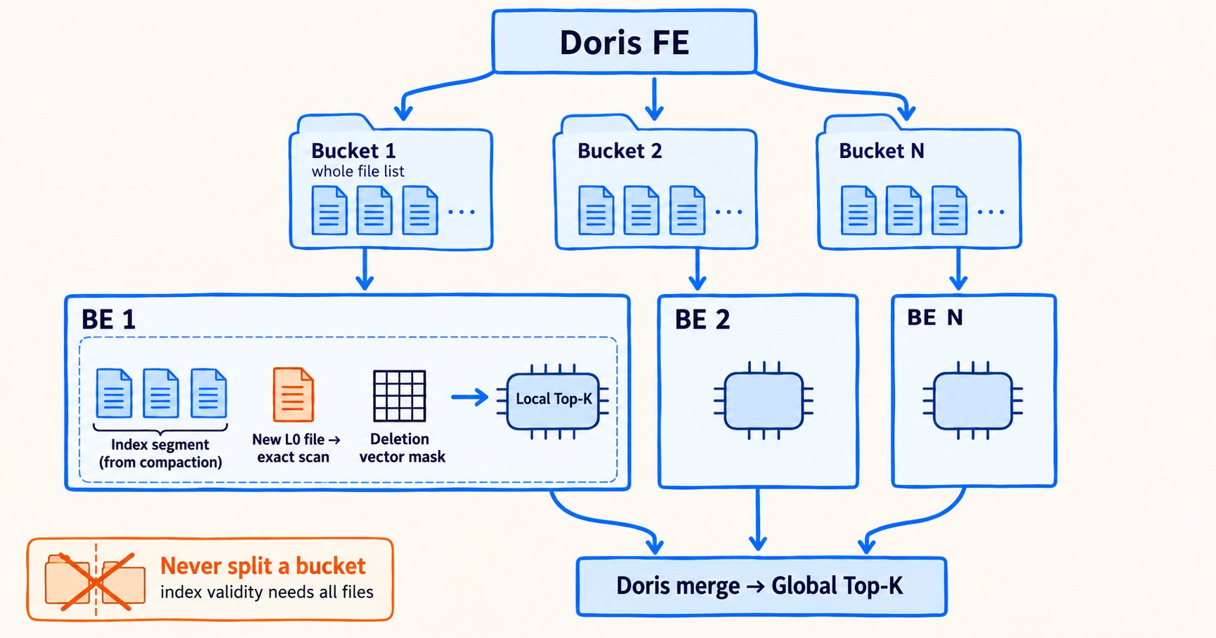
Figure 4: Each scan unit contains one complete bucket. The BE performs index retrieval, exact fallback, and deletion masking within that bucket. Doris then merges the Top-K across buckets.

2.3 Top-K pushdown and index-only scan

A standard vector-retrieval SQL query sorts rows by distance and returns the first K. The Doris FE uses an optimizer rule to recognize this pattern and rewrite the execution plan:

• Add a retrieval-score column to the scan node.
• Rewrite the distance expression in the original SQL as a conversion of this score, which avoids calculating the distance again.
• Change the sort order from ascending distance to descending score.
• When the vector column does not appear in the SELECT list, do not read the original vector column. This Index-Only Scan removes vector-column reads and transfers.

The optimizer applies the rule when all of the following conditions hold:

• The distance function matches the metric configured for the index.
• A vector index exists on the column.
• The SQL contains no aggregation or JOIN.

If any condition is not met, Doris uses a regular scan to preserve correct results.

The same rule handles queries with filters and pagination. The FE uses partition predicates for partition pruning and retains only buckets from relevant partitions. Predicates that can be converted into Paimon predicates are pushed down to Paimon Rust, which uses them to narrow the candidate set before retrieval. This provides pre-filtering. If the filter column is not indexed, the reader must scan that column. Doris functions such as length(a) > 1 cannot be pushed down, so Doris applies those predicates as post-filters to the retrieval results. For pagination, Doris combines OFFSET and LIMIT into a larger K value for pushdown, then applies the actual offset in the upper-level sort operator.

Users can write the same SQL they use for vector retrieval on Doris internal tables. They do not need to modify their queries to use vector indexes on Paimon tables.

Figure 5 shows how the optimizer identifies and rewrites the query.

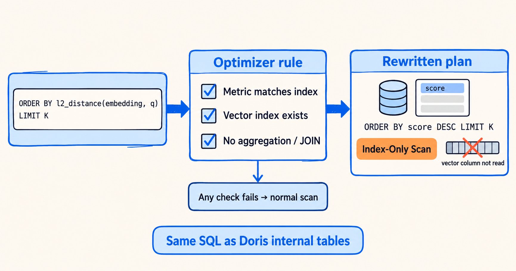
Figure 5: A vector Top-K query that meets all three conditions is rewritten to sort by score. If the query does not select the vector column, Doris does not read it. If any condition is unmet, Doris uses a regular scan.

2.4 Late materialization for large Top-K queries: separating retrieval from materialization

A typical Top-K SQL query looks like this:

select id, embedding from vec_table
order by l2_distance_approximate(embedding, [...])
limit <K>;

This SQL retrieves the id and embedding columns in a single scan and then performs retrieval. When K is small, this execution method adds little overhead.

When K is large, the cost of a single scan grows with it. Each bucket must read all user columns for K candidate rows, although the global merge will discard most of those rows. With K = 1 million and a 2,048-dimensional vector column, each candidate row carries 8 KB of vector data (2,048 × 4 bytes). As more candidates are discarded, more of those reads are wasted.

Kwai currently rewrites these queries as self-joins. A subquery performs retrieval and returns only IDs, then joins the original table to fetch vectors for the matching rows, as shown in Section 3.2. During the join, Doris pushes the candidate ID set down to the Paimon read layer. The reader uses this set to exclude unrelated files and row groups. It then uses Parquet page-level indexes to skip unrelated pages and materializes the vector column only for matching rows. In the Section 3.3 results, returning only IDs with Top-K = 1 million takes 7.9 to 8.0 seconds, while returning vectors as well takes 65 to 76 seconds. Most of that difference comes from reading and materializing vectors for the 1 million result rows. This approach works, but it requires users to rewrite their SQL.

The next execution plan is still under development. It separates retrieval and materialization into three stages:

• Candidate stage: Each BE performs retrieval on its assigned buckets without reading user columns and produces only a candidate set.
• Merge stage: All candidates are collected for global Top-K selection and reranking. The result is a list of rows to materialize, represented as data files and row ranges within those files. The list is grouped by data file, and matching row ranges are merged.
• Materialization stage: Read user columns only for rows in the row list.

The merge stage must run on a single node for algorithmic reasons. Reranking needs the global candidate set to calculate the correct Top-K, and grouping and merging row ranges also require the complete set. The aggregated candidate set is only on the order of megabytes, and this stage performs no hash or range repartitioning.

Figure 6 compares the one-pass scan with the three-stage plan.

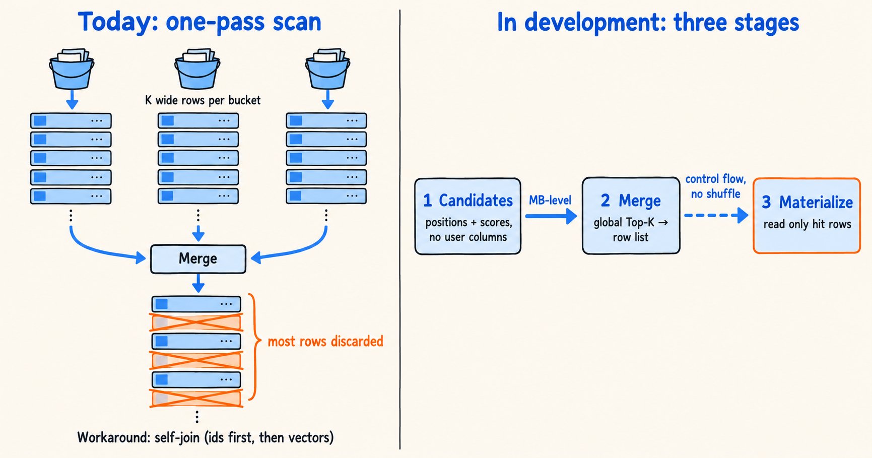
Figure 6: A one-pass scan makes every bucket read wide columns for K candidates. The three-stage plan first produces candidates alone, then materializes matching rows after the global Top-K step.

The expected benefits are:

• As Top-K grows, more candidate rows are discarded, so the system can avoid more wide-column reads.
• The materialization stage replaces the user-written self-join and removes that join from the execution plan.
• The FE uses a cost model to choose between the two forms automatically. Users do not need to know which form it selects or change their SQL.

Section 3 reports measured performance for the current one-pass form. Section 4 gives the current status of the three-stage implementation.

3. Performance: scale and results in Kwai's production environment

3.1 Deployment and benchmark methodology

Kwai already uses Doris external tables in production to query vector indexes on Paimon tables. The deployment is configured as follows:

Dimension	Choice
Table type	Paimon primary-key table (PK Table)
Vector storage	Inline, in the same table as the business columns
Vector index	IVF-RQ
Vector dimensions	2,048 (real production data)
Read path	Paimon Rust + Doris BE
Storage acceleration	Remote Alluxio cache
Query interface	Doris SQL
Cluster size	64 CU

The tests use the following dataset sizes:

Scale	Rows	Data volume	Buckets
Tens of millions	16 million	Approximately 150 GB	32
Hundreds of millions	128 million	Approximately 1.1 TB	256

3.2 Two query types

The first query type returns only business identifiers. The vector index produces the Top-K directly:

select id
from vec_table
order by l2_distance_approximate(embedding, [...]) /* 2,048-dimensional query vector */
limit <K>; -- K is 100, 10,000, or 1,000,000

This is a typical Index-Only Scan test case. It primarily measures the cost of retrieval itself.

The second query type returns both business identifiers and vectors. With the current implementation, users rewrite these queries as self-joins. A subquery retrieves the Top-K IDs, then joins the original table to fetch vectors for the matching rows:

select t1.id, embedding
from (select id, embedding from vec_table) t1
join (
select id
from vec_table
order by l2_distance_approximate(embedding, [...]) /* 2,048-dimensional query vector */
limit <K>
) t2 on t1.id = t2.id;

The "Business identifier + vector" column in the Section 3.3 table uses this self-join SQL. It primarily measures the cost of reading and materializing the vector column. After the three-stage plan described in Section 2.4 is implemented, users will be able to write the same query directly as:

select id, embedding
from vec_table
order by l2_distance_approximate(embedding, [...]) /* 2,048-dimensional query vector */
limit <K>; -- K is 100, 10,000, or 1,000,000

The materialization stage will then replace the self-join, and the SQL will be identical to a query against a Doris internal table.

3.3 Measured results from tens of millions to hundreds of millions of vectors

The following table reports query performance and recall for different parameter combinations. Both latency columns measure end-to-end latency. Queries that return only business identifiers use the first SQL statement in Section 3.2. Queries that also return vectors use the self-join SQL. The values are representative results from individual queries:

Vector count	Top-K	Business identifier	Business identifier + vector	Recall
16 million	100	1.4 seconds	2.4 seconds	96.0%
128 million	100	1.8 seconds	2.5 seconds	97.0%
16 million	10,000	1.8 seconds	2.3 seconds	99.2%
128 million	10,000	2.0 seconds	4.6 seconds	98.5%
16 million	1 million	7.9 seconds	65 seconds	97.8%
128 million	1 million	8.0 seconds	76 seconds	99.6%

The table supports two conclusions:

• Index-retrieval latency changes little with data scale. When the row count grows from 16 million to 128 million, latency for returning only business identifiers increases by 0.4 seconds, 0.2 seconds, and 0.1 seconds across the three Top-K settings, respectively.
• When Top-K = 1 million, vector-column materialization is the bottleneck, not retrieval.

These are representative results from individual queries. The table does not cover QPS.

3.4 Comparing vector retrieval on Paimon tables and Doris internal tables

Kwai also compared vector retrieval on Paimon tables with retrieval on Doris internal tables. The team loaded the same Paimon data into Doris internal tables and queried it through Doris's own vector indexes. The following table gives the results.

Vector count	Top-K	Returned data	Doris internal table (local cache)	Paimon external table (Alluxio)	External / internal
16 million	100	Business identifier	0.49 seconds	1.4 seconds	2.86×
16 million	100	Business identifier + vector	0.7 seconds	2.4 seconds	3.43×
128 million	100	Business identifier	0.7 seconds	1.8 seconds	2.57×
128 million	100	Business identifier + vector	0.8 seconds	2.5 seconds	3.13×
16 million	10,000	Business identifier	0.58 seconds	1.8 seconds	3.10×
16 million	10,000	Business identifier + vector	1.4 seconds	2.3 seconds	1.64×
128 million	10,000	Business identifier	0.7 seconds	2.0 seconds	2.86×
128 million	10,000	Business identifier + vector	1.1 seconds	4.6 seconds	4.18×
16 million	1 million	Business identifier	7.2 seconds	7.9 seconds	1.10×
16 million	1 million	Business identifier + vector	61 seconds	65 seconds	1.07×
128 million	1 million	Business identifier	7.2 seconds	8.0 seconds	1.11×
128 million	1 million	Business identifier + vector	56 seconds	76 seconds	1.36×

• External-table latency is 1.07 to 4.18 times internal-table latency. When the query returns only business identifiers, the absolute difference is 0.7 to 1.3 seconds.
• At Top-K = 1 million, the difference narrows to 1.07 to 1.36 times. Most of the latency at this setting comes from row lookup and materialization. Both sides read the same amount of data, which reduces the effect of cache location.

Figure 7 summarizes the results measured by Kwai.

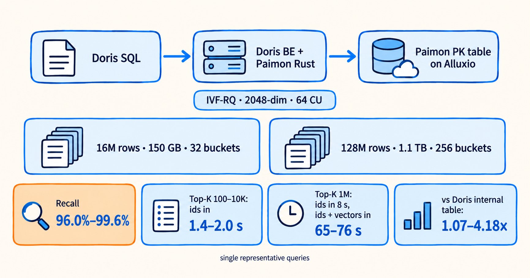
Figure 7: Recall is 96.0% to 99.6% at both scales. Queries that return only business identifiers finish within 2.0 seconds for Top-K values up to 10,000. At Top-K = 1 million, materialization accounts for most of the latency.

Internal tables perform better, but returning only business identifiers adds just 0.7 to 1.3 seconds of query latency in absolute terms. In return, Kwai gets the following operational benefits:

• Better data freshness between writing data to Paimon and making it searchable.
• Unified storage without redundant data copies.
• No compute-resource overhead for transferring and converting data between different systems.
• No separate access-control and governance systems to maintain.

4. Results and roadmap of joint development by the Doris and Paimon communities

Kwai, the Apache Doris community, and the Apache Paimon community developed this read path together. Kwai has contributed more than 120 PRs to the Apache Paimon and Apache Paimon Rust communities. The Doris-side changes are planned for merger into the Doris community within the next two months.

Kwai is also working on the following changes to improve vector retrieval performance when Doris queries Paimon:

• Three-stage late materialization: The plan described in Section 2.4 separates candidate retrieval from vector-column materialization. At operating points such as Top-K = 1 million, the system will stop reading wide columns for candidate rows that are later discarded. Users will also no longer need to write self-joins manually.
• Local index caching: Add local disk and memory caches within the calling process, with Doris providing consistent-hash distribution.
• Full-text retrieval and Hybrid Search: The full-text retrieval path is already complete on the Paimon side. After the Doris-side integration is complete, users will be able to combine structured filtering, keyword matching, and semantic retrieval on the same lake table.
• Completing retrieval semantics: Add similarity-range retrieval. Kwai has begun an internal grayscale rollout and plans to contribute the feature to the community after large-scale production validation. Retrieval parameters will also become overridable per query instead of remaining limited to table-level configuration.

Learn more

The multimodal lakehouse capabilities for Paimon, Iceberg, Lance, and other formats have been merged into the Doris 4.2 release branch. They are scheduled for official release with version 4.2 at the end of September.