
26 posts tagged with "Tech Sharing"

View All Tags
Blog/Tech Sharing

Kang, Apache Doris PMC Member

The author previously presented this topic at the VeloDB Webinar. This article expands on that presentation by providing more detailed comparative information, including test data and in-depth technical explanations: https://www.youtube.com/embed/qnxX-FOd8Wc?si=TcEF_w-XhqgQyP4A

In the past year, there's an increasing number of users looking to use Apache Doris as an alternative to Elasticsearch, so I'd like to provide an in-depth comparison of the two to serve as a reference for users.

Apache Doris is a real-time data warehouse commonly used for observability, cyber security analysis, online reports, customer profiles, data lakehouse and more. Elasticsearch is more like a search engine, but it is also widely used for data analytics, so there's an overlap in their use cases. The comparison in this post will focus on the real-time analytics capabilities of Apache Doris and Elasticsearch from a user-oriented perspective:
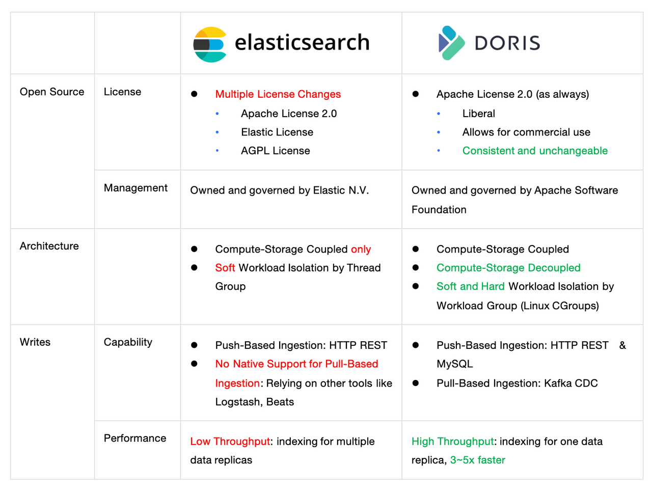
  1. Open source
  2. System architecture
  3. Real-time writes
  4. Real-time storage
  5. Real-time queries

Open source

The license decides the level of openness of an open source product, and further decides whether users will be trapped in a vendor lock-in situation.

Apache Doris is operated under the Apache Software Foundation and it is governed by Apache License 2.0. This is a highly liberal open source license. Anyone can freely use, modify, and distribute Apache Doris in open source or commercial projects.

Elasticsearch has undergone several changes in licenses. It was subject to Apache License 2.0 at the very beginning. Then in 2021, it switched to the Elastic License and SSPL, mostly because some cloud service providers were providing Elasticsearch as a managed service. The Elastic company tried to protect its business interests and moved to the Elastic License in order to restrict certain commercial use. And then in 2024, Elasticsearch announced that "Elasticsearch Is Open Source. Again!" by adding the AGPL License. This license has less restrictions on cloud providers.

The difference in licenses reflects the differing ways in which the two open-source projects are managed and operated. Apache Doris is operated under the Apache Software Foundation and adheres to "the Apache Way" and maintains vendor neutrality. It will always be under Apache License and maintain a high level of openness. Elasticsearch is owned and run by the Elastic company, so it is free to change its license based on the changing needs of the company.

System architecture

The system architecture of Apache Doris and Elasticsearch is relevant to how users can deploy them and the software/hardware prerequisites that must be met.

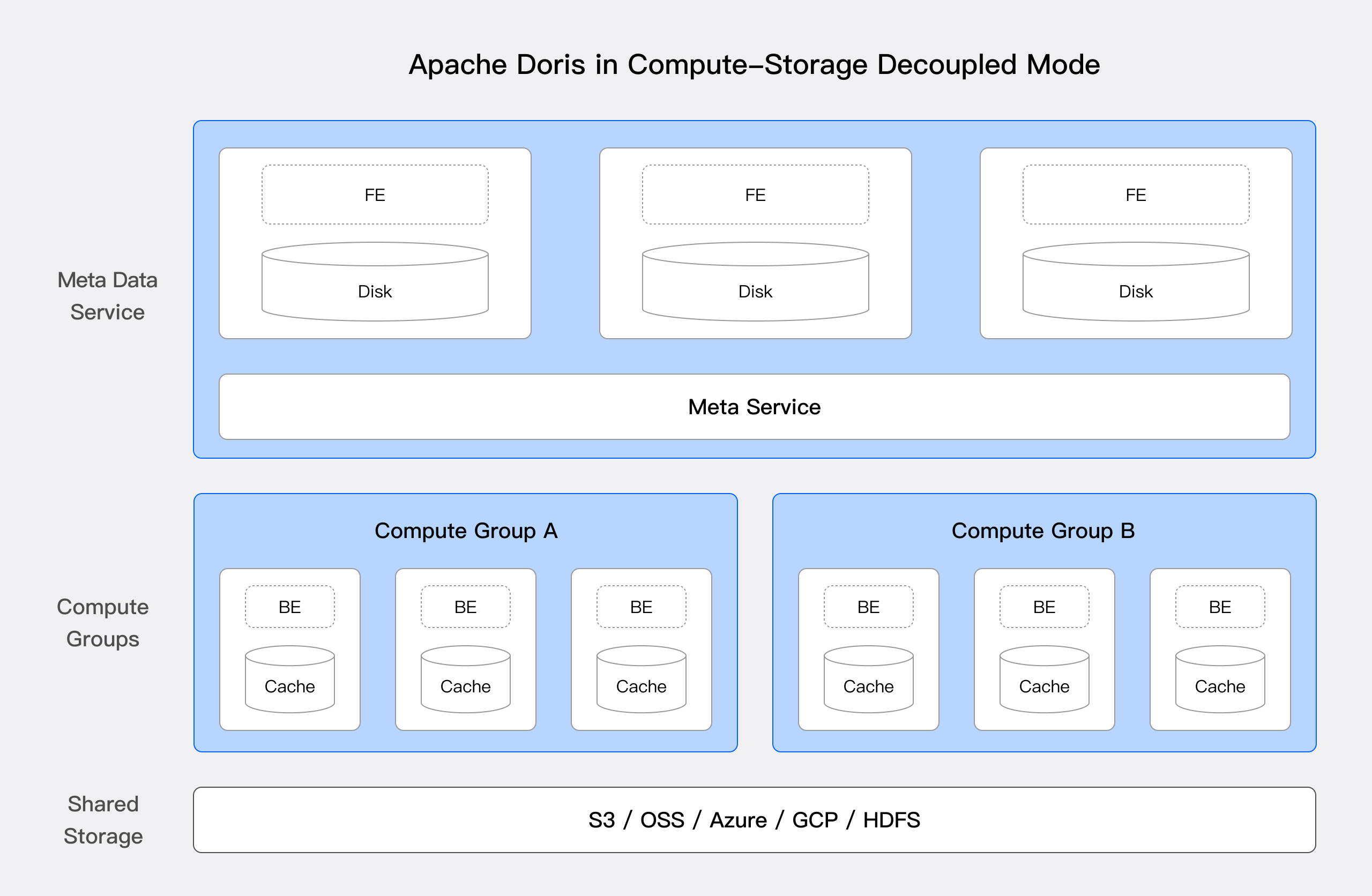
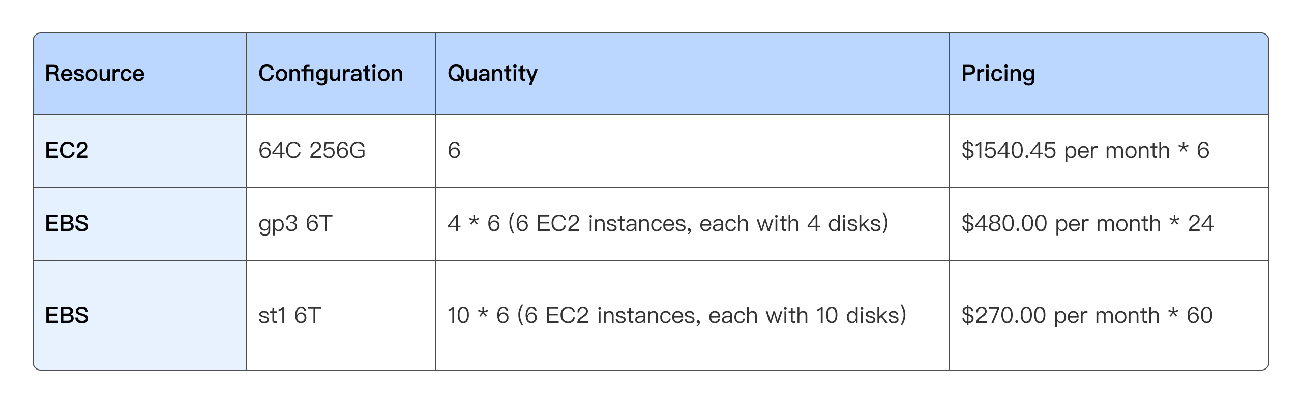
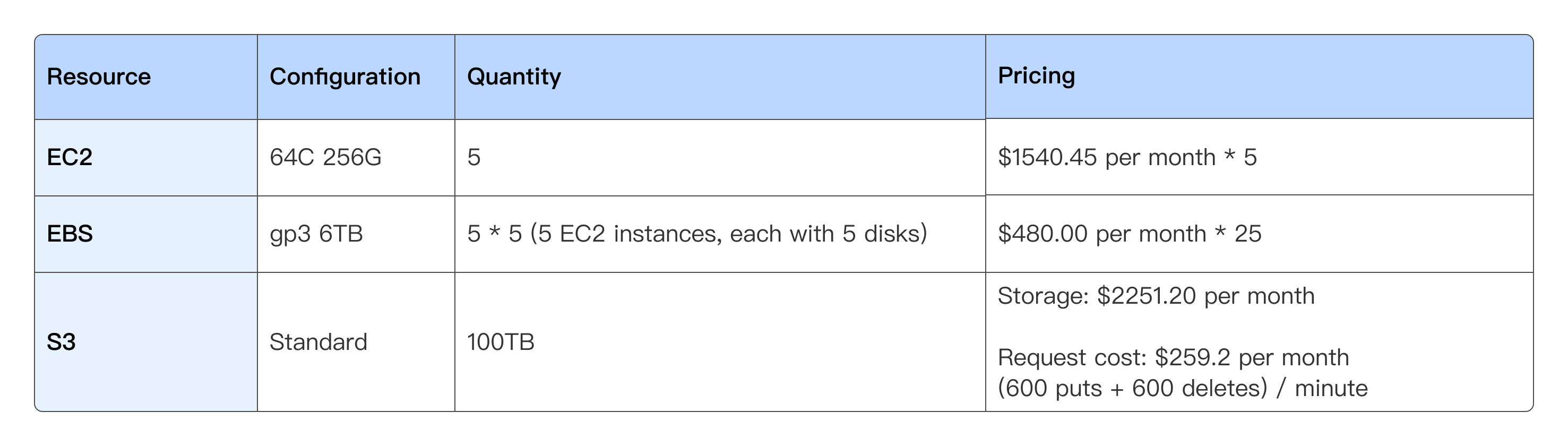
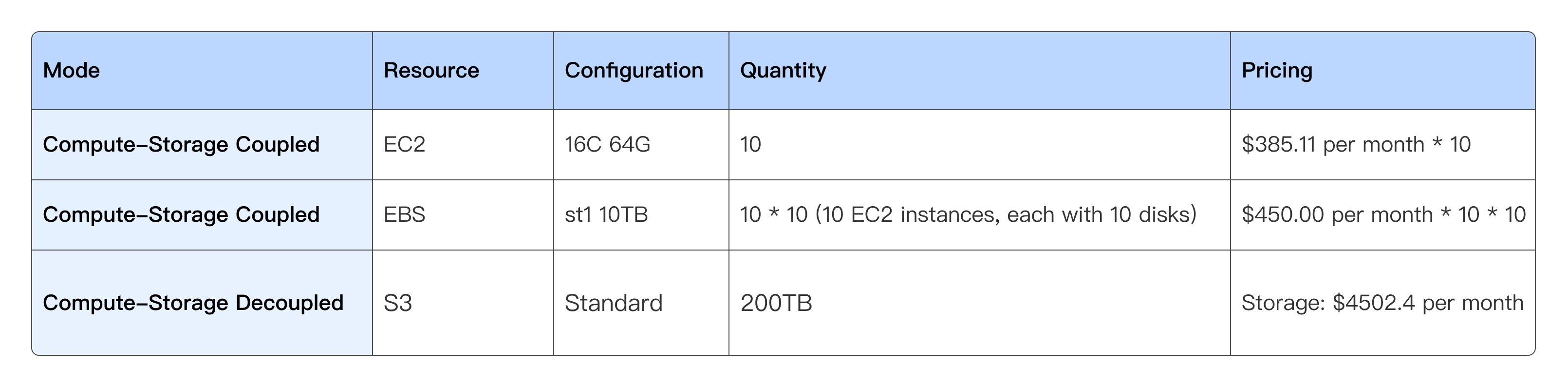
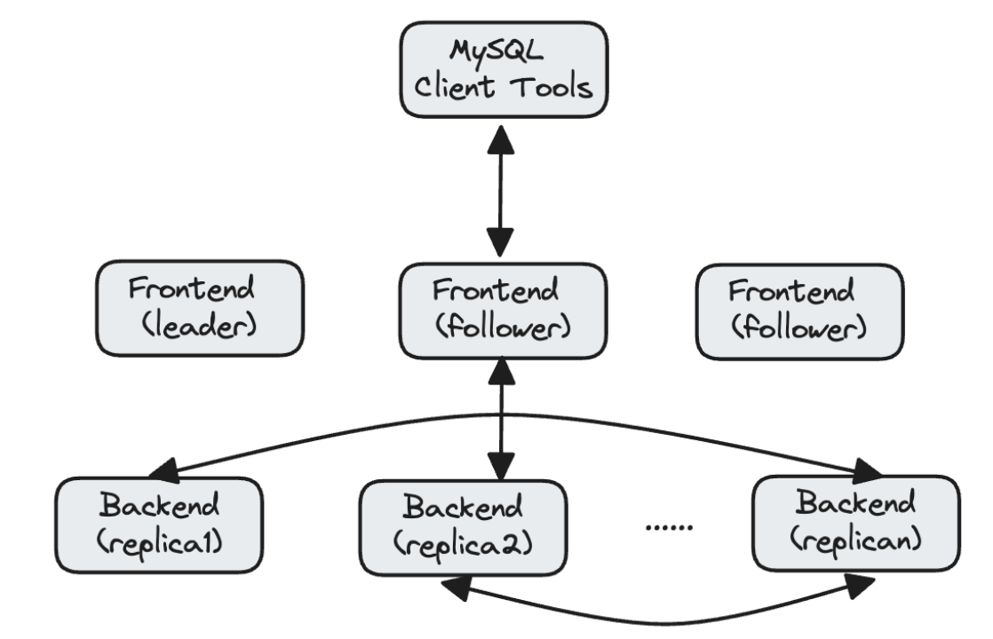
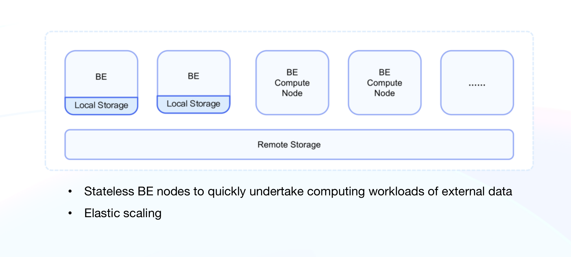
Apache Doris supports various deployment models, especially after the release of verion 3.0. It can be deployed on-premise the traditional way, which means compute and storage are integrated within the same hardware. It can also be deployed with compute and storage decoupled, providing higher flexibility and elasticity.

System architecture.jpeg

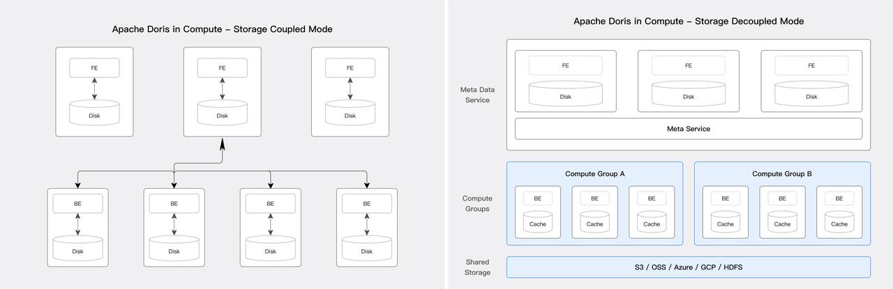
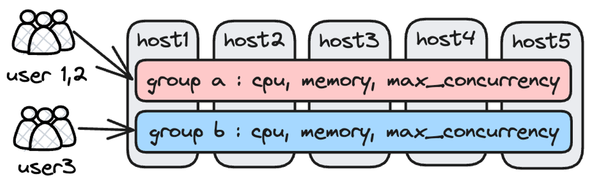
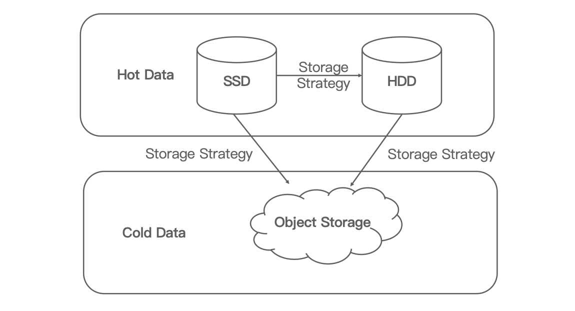
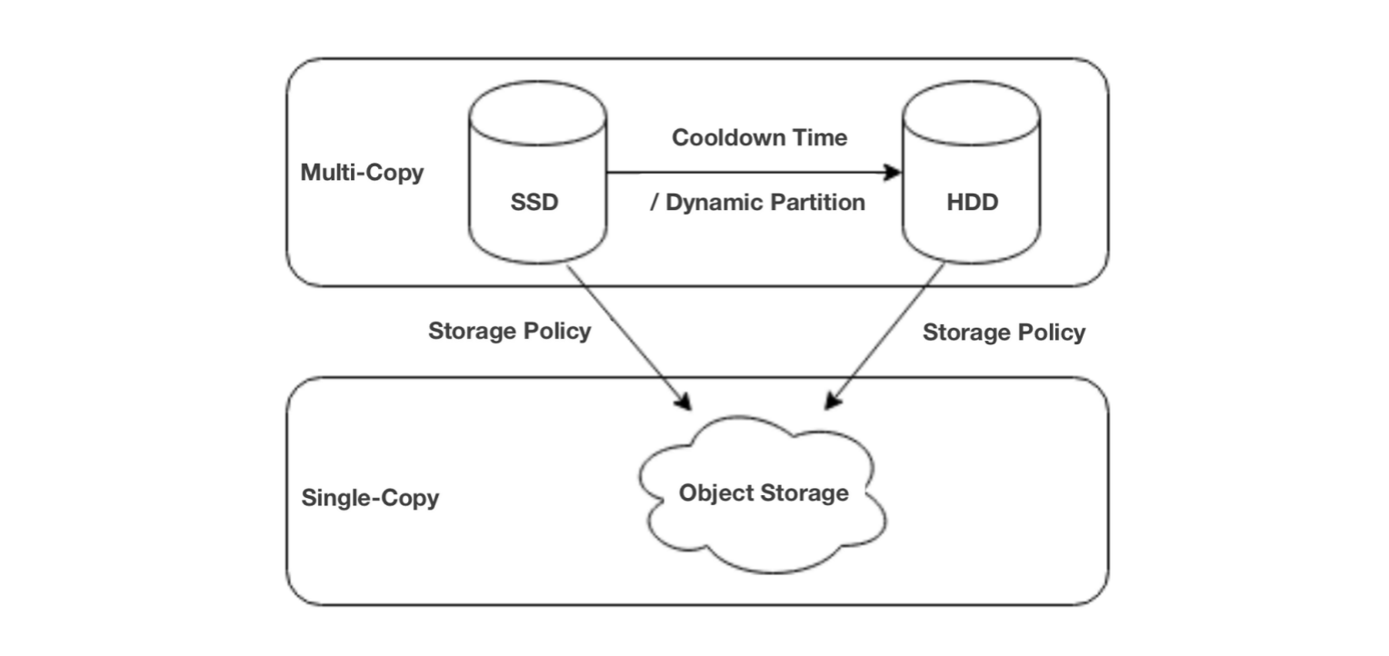
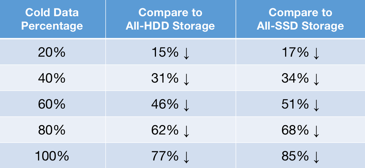
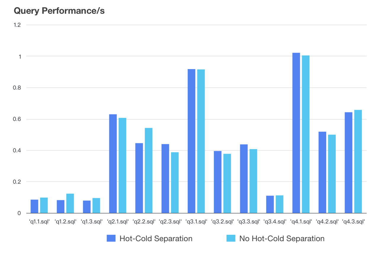
Apache Doris enables the isolation of computing workloads, which makes it well-suited for multi-tenancy. In addition to decoupling compute and storage, it also provides tiered storage so you can choose different storage medium for your hot and cold data.

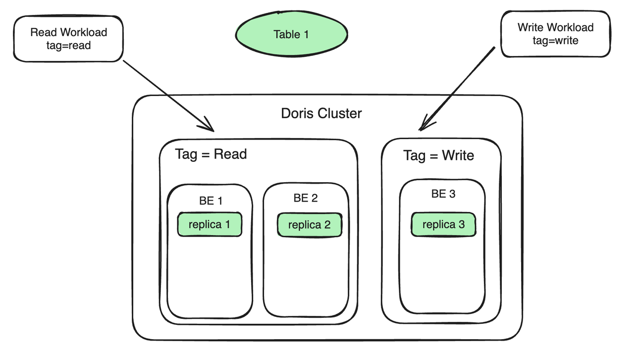
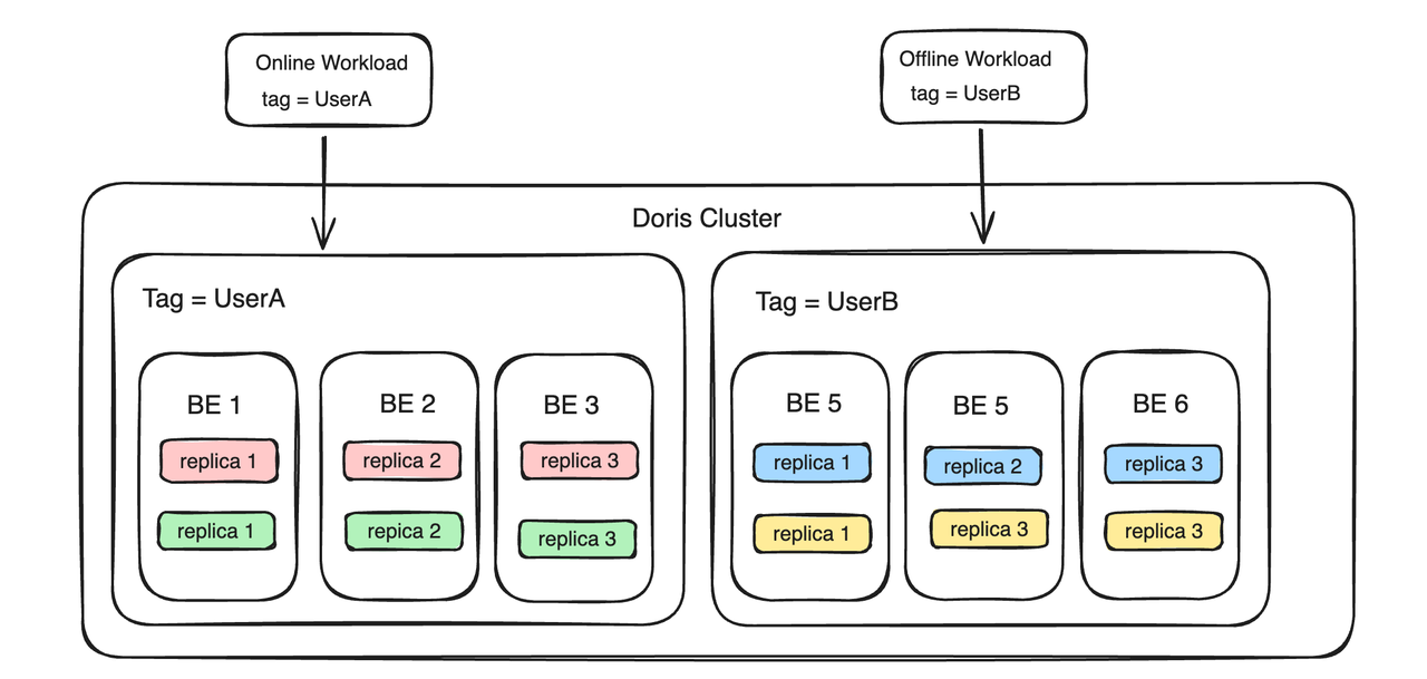
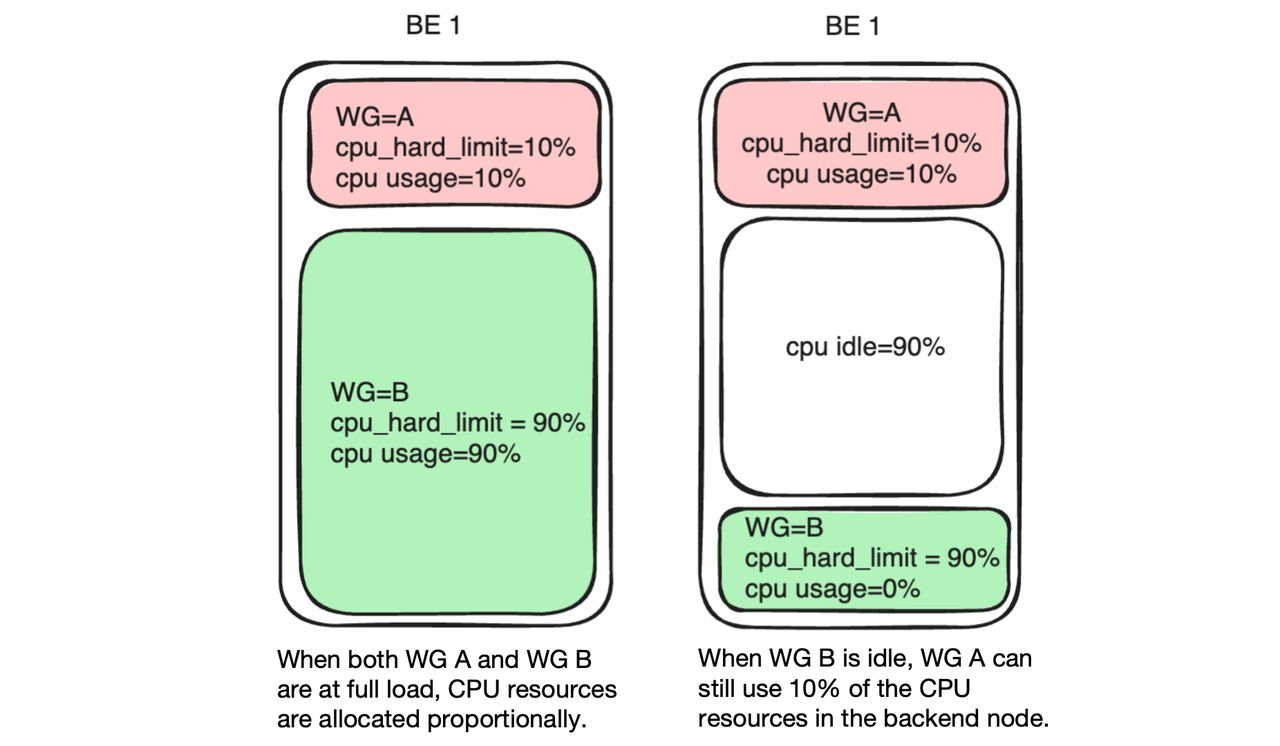
For workload isolation, Apache Doris provides the Compute Group and Workload Group mechanism.

System architecture-2.png

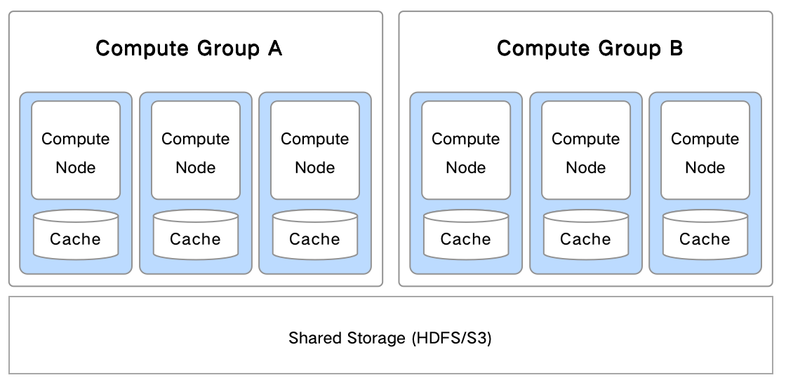
Compute Group is a mechanism for physical isolation between different workloads in a compute-storage decoupled architecture. One or more BE nodes can form a Compute Group.

System architecture-3.png

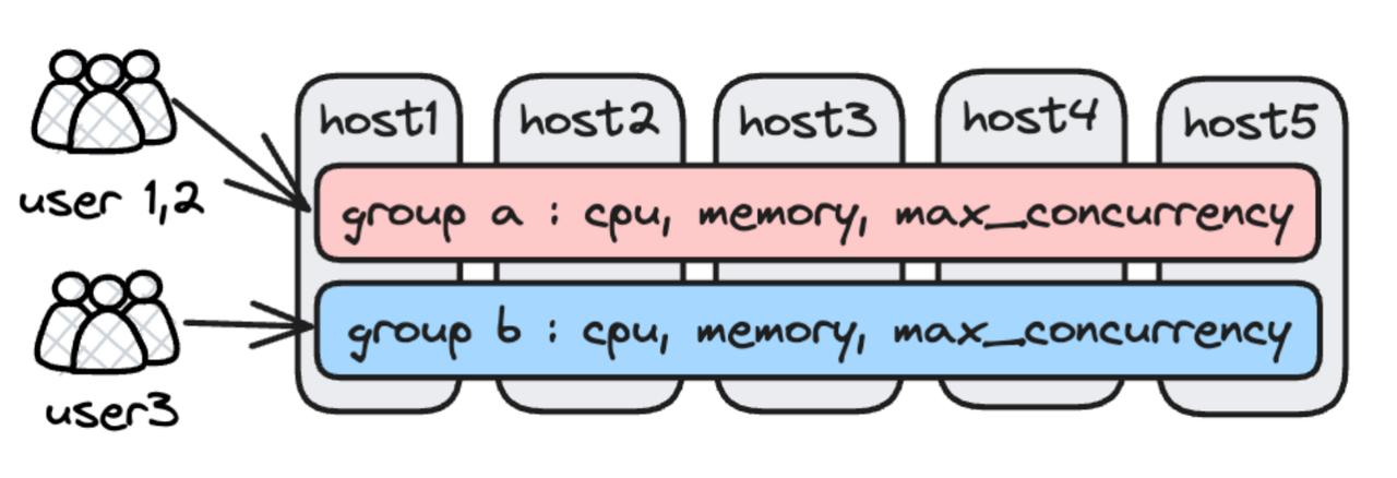
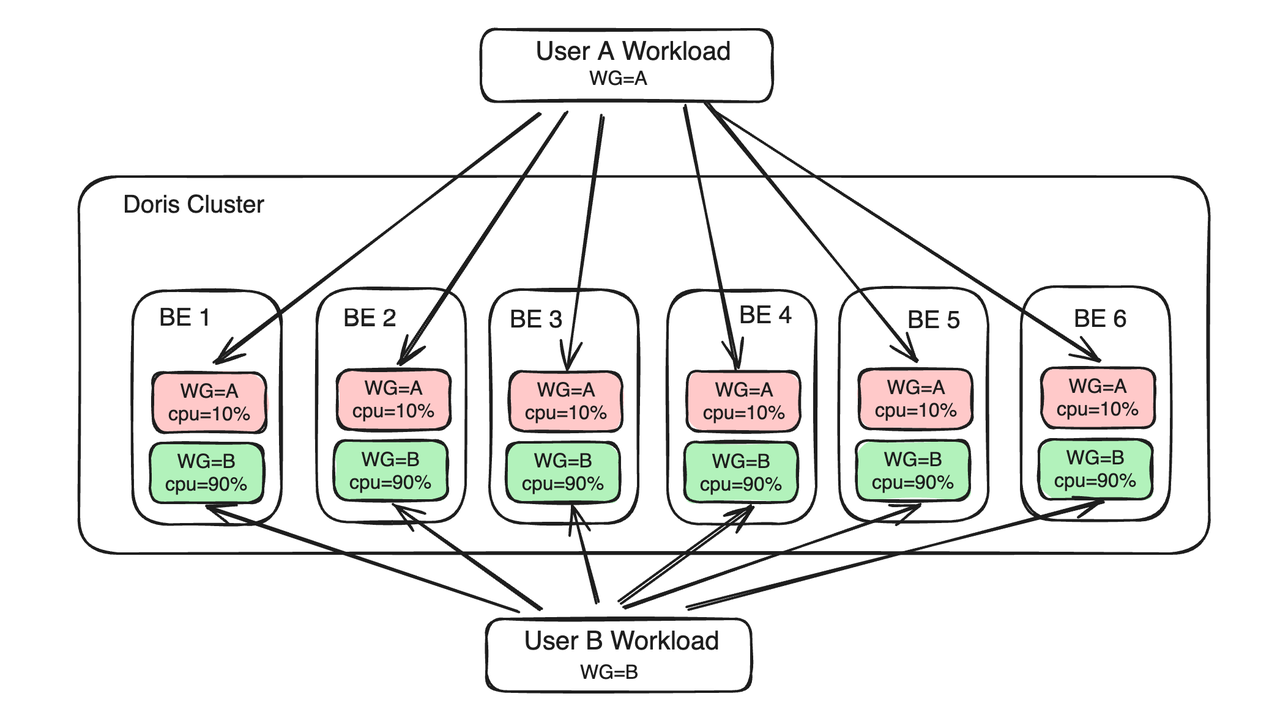
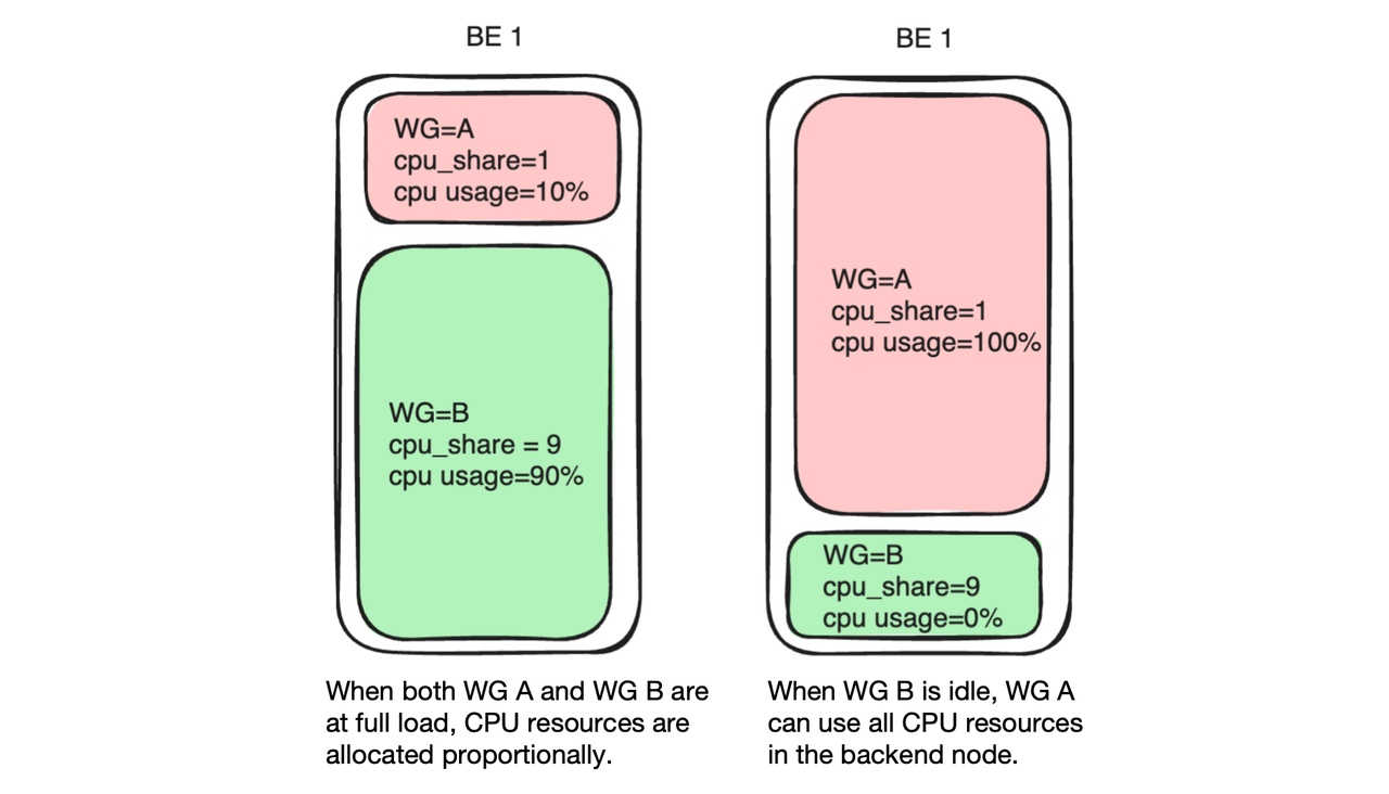
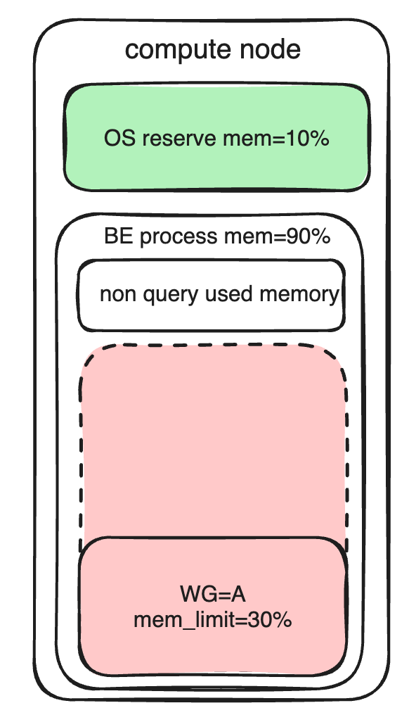
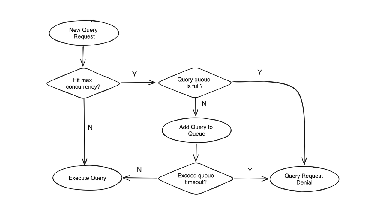
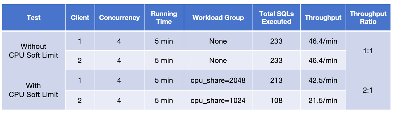
Workload Group is an in-process mechanism for isolating workloads. It achieves resource isolation by finely partitioning or limiting resources (CPU, IO, Memory) within the BE process, which is implemented by Linux CGroup and offers strict hard isolation.

Elasticsearch supports on-premise and cloud deployment. It does not support compute-storage decoupling. Elasticsearch implements workload isolation by Thread Groups, which provides limited soft resource isolation.

Real-time writes

The next step after deploying the system is to write data into it. Apache Doris and Elasticsearch are very different in data ingestion.

Write capabilities

Normally there are two ways to write real-time data into a data system. One is push-based, and the other is pull-based. A push-based method means users actively push the data into the database system, such as via HTTP. A pull-based method, for example, is where database system pulls data from data source such as Kafka message queue.

Elasticsearch supports push-based ingestion, but it requires Logstash to perform pull-based data ingestion, making it less convenient.

As for Apache Doris, it supports both push-based method (HTTP Stream Load) and pull-based method (Routine Load from Kafka, Broker Load from object storage and HDFS). In addition, output plugins for Logstash and Beats are available to enable seamless data ingestion from Logstash or Beats into Doris.

In addition, Doris provides a special write transaction mechanism. By setting a label for a batch of data through the Load API, attempting to re-load a label that has been successfully load before will result in an error, thereby achieving data deduplication. This mechanism ensures that data is written without loss or duplication without relying on the uniqueness of primary keys at the storage layer. Additionally, having a unique label for each batch of data offers better performance compared to having a unique primary key for each individual record.

Write performance

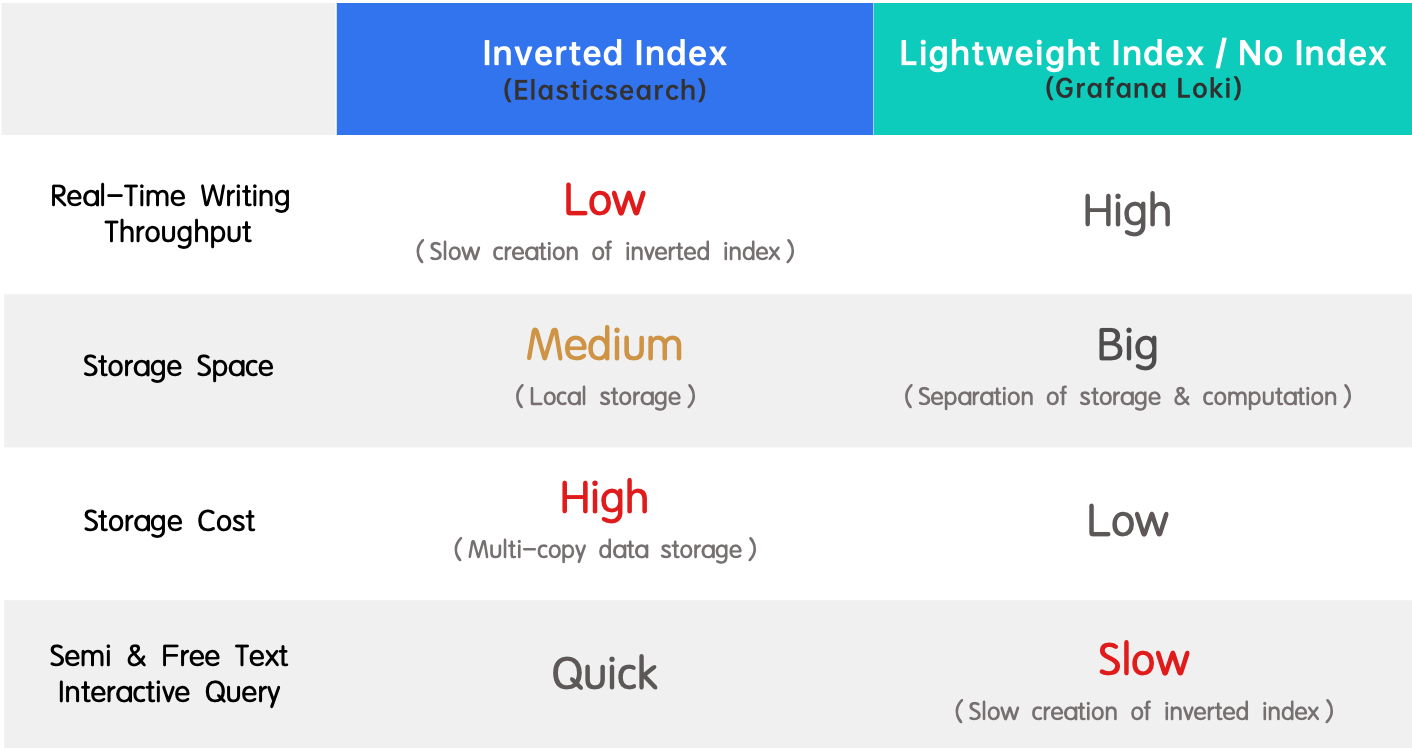
Apache Doris, as a real-time data warehouse, supports real-time data writes and updates. One of the standout features of Doris is its incredibly high write throughput. This is because the Doris community has put a lot of effort in optimizing it for high-throughput writes such as vertorized writting and single replica indexing.

On the other hand, the low write throughput of Elasticsearch is a well-known pain point. This is due to Elasticsearch's needs to generate complex inverted index on multiple replicas, causing a lot of overheads.

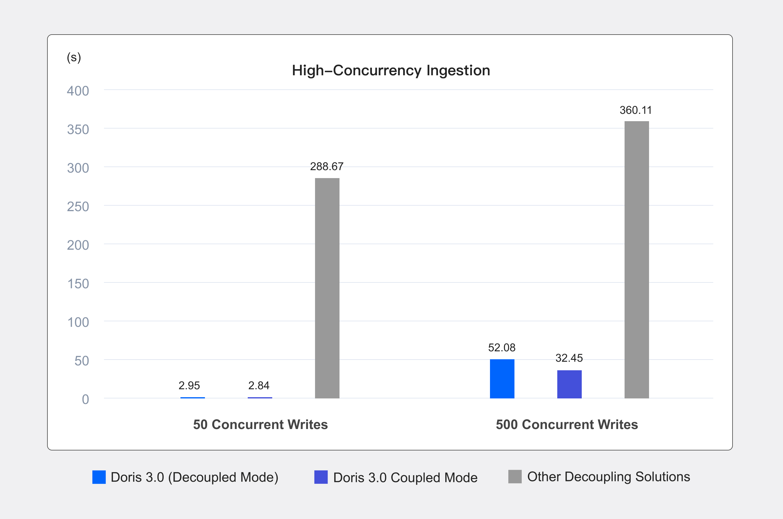
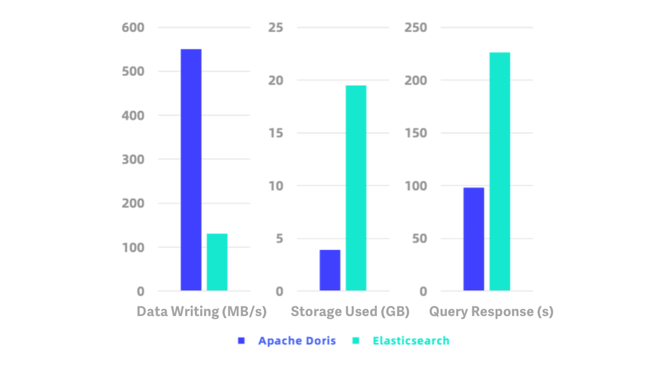
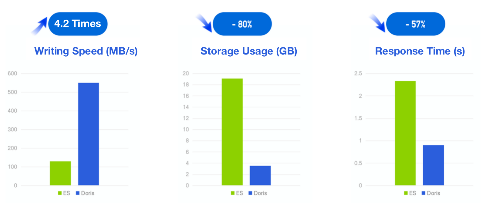
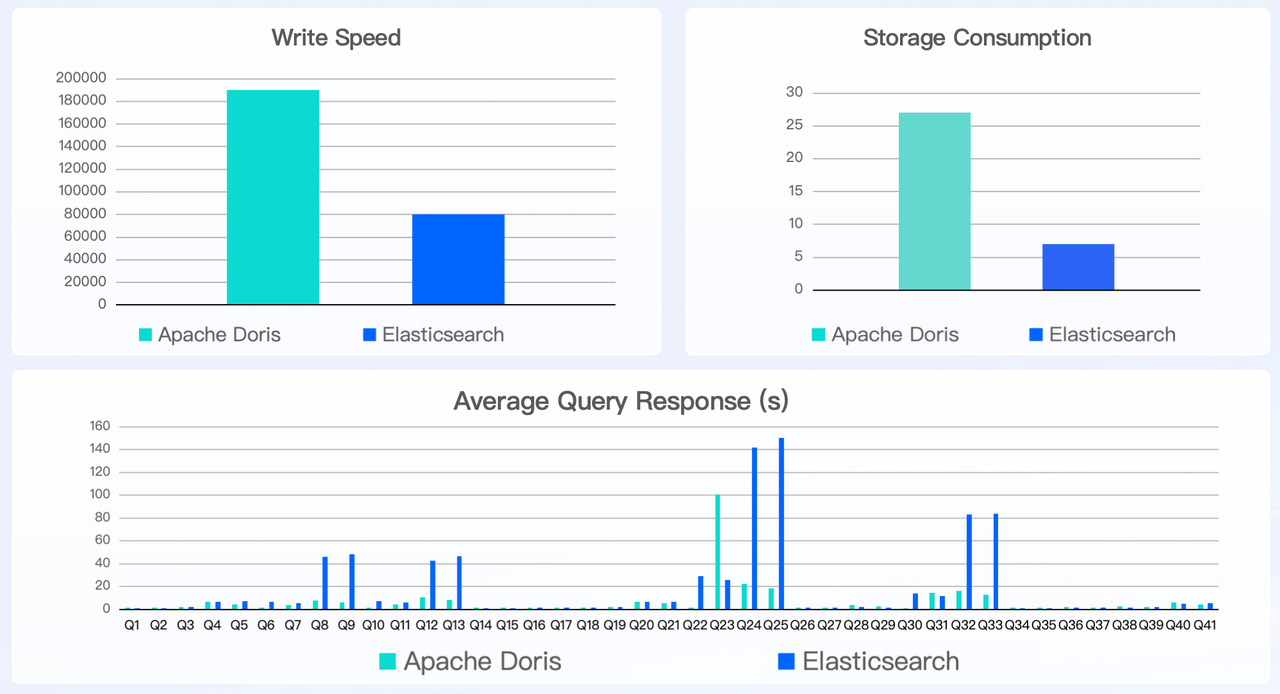
We compare the write performance of Doris and Elasticsearch using Elasticsearch's official benchmark httplogs, under the same hardware resources and storage schema (including field types and inverted indexes). The test environment and results are as follows:

write performance.png

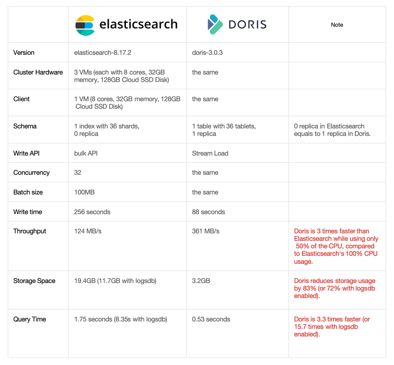
Under the premise of creating the same inverted index, Apache Doris delivers a much higher write throughput than Elasticsearch. This is due to some key advancements in performance optimization, including:

  1. Doris is implemented in C++, which is more efficient than Elasticsearch's Java implementation.
  2. The vectorized execution engine of Doris fully utilizes CPU SIMD instructions to accelerate both data writing and inverted index building. Its columnar storage also facilitates vectorized execution.
  3. The inverted index of Doris is simplified for real-time analytics scenarios, eliminating unnecessary storage structures such as forward indexes and norms.

Real-time storage

Storage format and cost

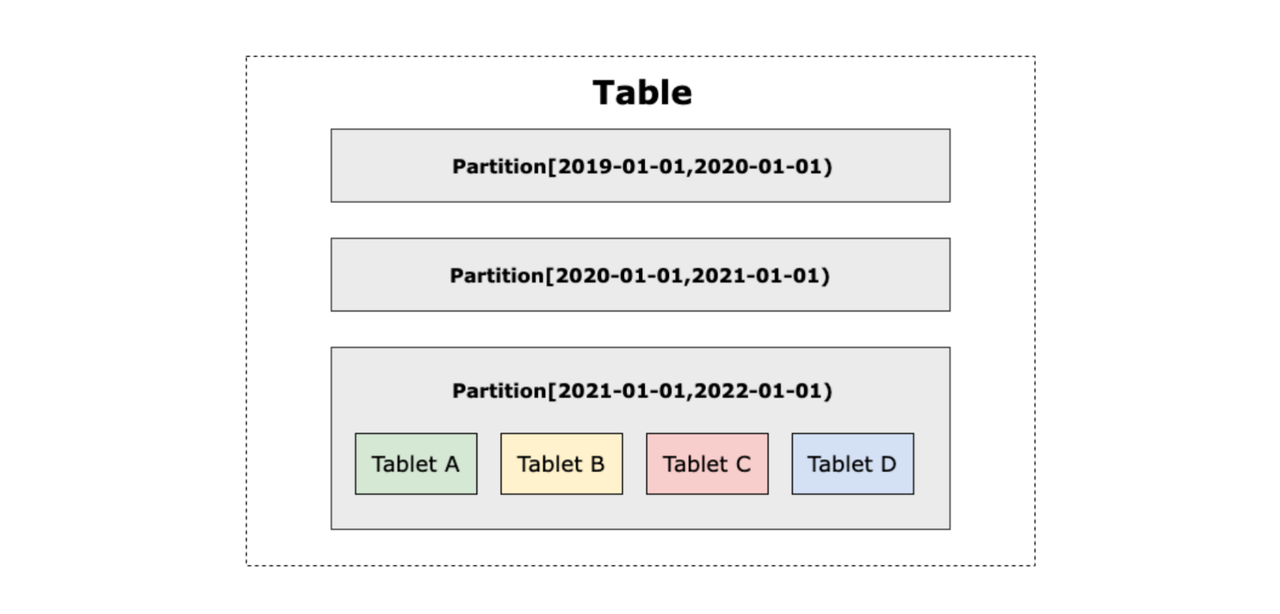
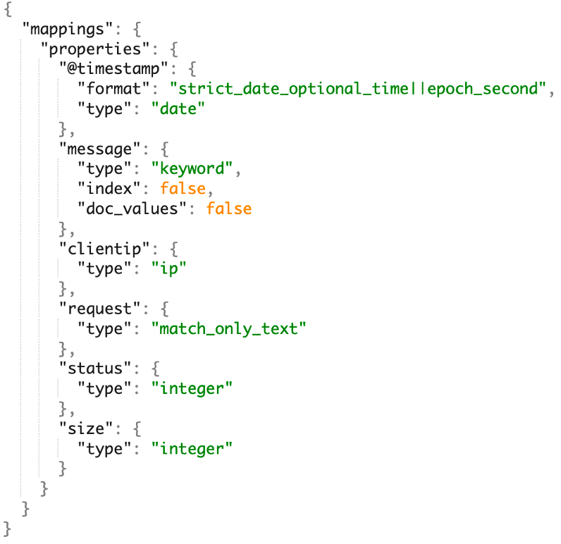
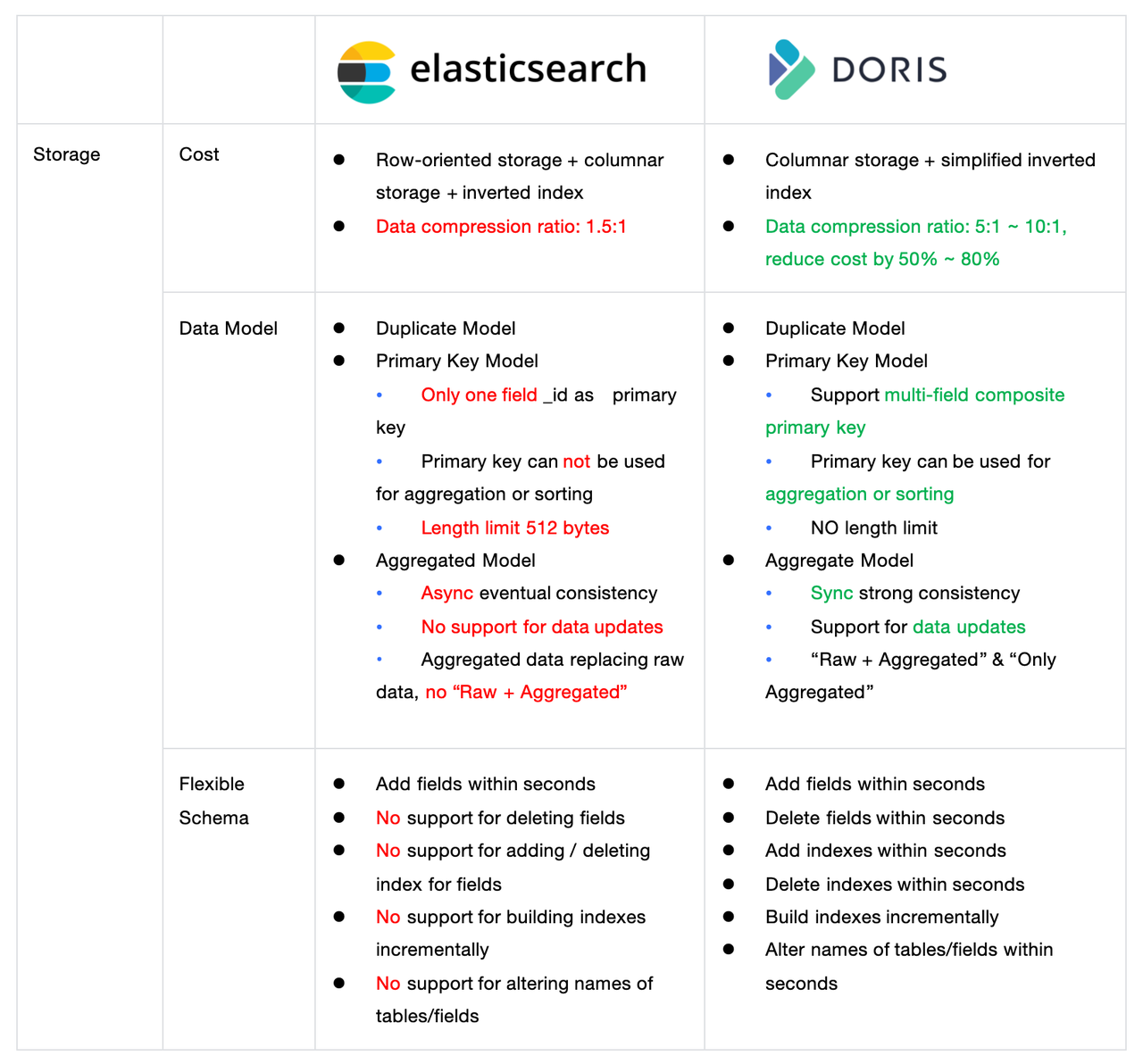
As a real-time data warehouse, Doris adheres to the typical relational database model, with a storage hierarchy that includes catalog, database, and table levels. A table consists of one or more columns, each with its own data type, and indexes can be created on the columns.

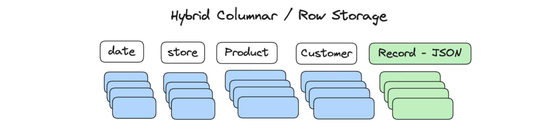
By default, Doris stores tables in a columnar format, meaning that data for a single column is stored in contiguous physical files. This not only achieves a high compression ratio but also ensures high query efficiency in analysis scenarios where only certain columns are accessed, as only the required data is read and processed. Additionally, Doris supports an optional row storage format to accelerate detailed point queries.

In Elasticsearch, data is stored in Lucene using a document model. In this model, an Elasticsearch index is equivalent to a database table, the index mapping corresponds to the database table schema, and fields within the index mapping are akin to columns in a database, each with its own type and index type.

By default, Elasticsearch uses row-based storage (the _source field), where each field has an associated inverted index created for it, but it also supports optional columnar storage (docvalue). Generally, row-based storage is essential in Elasticsearch because it lays the foundation for raw detailed data queries.

Storage space consumption, or more straightforward, storage cost, is a big concern for users. This is another pain point of Elasticsearch - it creates huge storage costs.

Apache Doris community have made a lot of optimizations and successfully reduced the storage cost significantly. We have put a lot of work to simplify inverted index, which is supported in Doris since version 2.0, and it now takes up much less space. Doris supports the ZSTD algorithm, which is much more efficient than GZIP and LZ4, and it can reach a data compression ratio of 5:1 ~ 10:1. Since the compression ratio of Elasticsearch is usually about 1.5:1, Doris is 3~5 times more efficient than Elasticsearch in data compression.

As demonstrated in the httplogs test results table above, 32GB of raw data occupies 3.2GB in Doris, whereas Elasticsearch defaults to 19.4GB. Even with the latest logsdb optimization mode enabled, Elasticsearch still consumes 11.7GB. Compared to Elasticsearch, Doris reduces storage space by 83% (73% with logsdb enabled).

Table model

Apache Doris provides three data models. As for Elasticsearch, I put it as "one and two half" models because it only provides limited support for certain data storage models. I will get to them one by one.

  • The first is the Duplicate model, which means it allows data duplication. This is suitable for storing logs. Both Doris and Elasticsearch support this model.

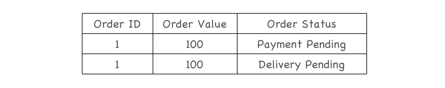
  • The second is the primary key model. It works like OLTP databases, which means the data will be deduplicated by key. The primary key model in Doris provides high performance and many user-friendly features. Just like many databases, you can define one or multiple fields as the primary and unique key.

    • However, in Elasticsearch, you can only use a special field _id as the unique identifier for a document (a row in database). Unlike database primary key, there are many limitations for it.

    • The _id field can not be used for aggregation or sorting

    • The _id field can not be larger than 512 bytes

    • The _id field can not be multiple fields, so you will need to combine the multiple fields into one before you can use them as the primary key, but the length of the combined _id can still not exceed 512 bytes.

  • The third is the aggregation model, which means data will be aggregated or rolled up.

In its early stages, Elasticsearch provided the rollup feature through the commercial X-Pack plugin, allowing users to create rollup jobs that configured dimensions, metric fields, and aggregation intervals for rollup indexes based on a base index. However, X-Pack rollup had several limitations:

  1. Data Asynchrony: Rollup jobs ran in the background, meaning the data in the rollup index was not synchronized in real time with the base index.
  2. Specialized Query Requirement: Queries targeting rolled-up data required dedicated rollup queries, and users had to manually specify the rollup index in their queries.

Perhaps these reasons explain why Elasticsearch has deprecated the use of rollup starting in version 8.11.0 and now recommends downsampling as an alternative. Downsampling eliminates the need to specify a separate index and simplifies querying, but it also comes with its own constraints:

  1. Time-Series Exclusive: Downsampling is only applicable to time-series data, relying on time as the primary dimension. It cannot be used for other data types, such as business reporting data.
  2. Index Replacement: A downsampled index replaces the original index, meaning aggregated data and raw data cannot coexist.
  3. Read-Only: Downsampling can only be performed on the original index after it transitions to a read-only state. Data actively being written (e.g., real-time ingestion) cannot undergo downsampling.

As a real-time data warehouse excelling in aggregation and analytics, Doris has supported aggregation capabilities since its early use cases in online reporting and analytics. It offers two flexible mechanisms:

  1. Aggregation Table Model:
    • Data is directly aggregated during ingestion, eliminating the storage of raw data.
    • Only aggregated results are stored, drastically reducing storage costs.
  2. Aggregated Materialized Views/ Rollup:
    • Users can create aggregated materialized views on a base table. Data is written to both the base table and the materialized view simultaneously, ensuring atomic and synchronized updates.
    • Queries target the base table, and the query optimizer automatically rewrites queries to leverage the materialized view for accelerated performance.

This design ensures real-time aggregation while maintaining query flexibility and efficiency in Doris.
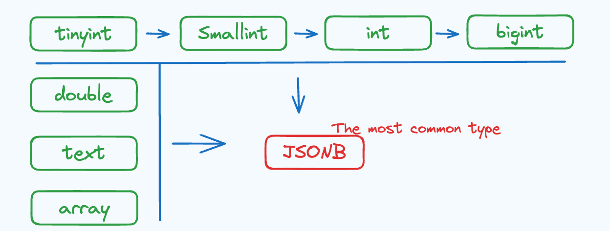
Flexible schema

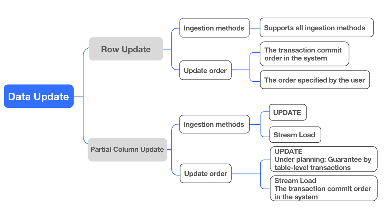
In most cases, especially for online business scenarios, users often need to update or modify the data schema. Elasticsearch supports flexible schema, but it only allows users to dynamically add columns.

Flexible schema.png

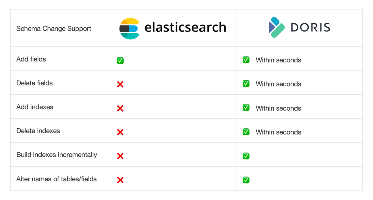
When you write JSON data into Elasticsearch, if the data contains a new field which is not in index mapping, Elasticsearch will create a new field in the schema through dynamic mapping, so you don't need to change the schema beforehand, like you have to do in traditional databases. However, in Elasticsearch, users cannot directly delete a field of the schema. For that, you will need a reindex operation that reads and writes the entire index in Elasticsearch.

In addition, Elasticsearch does not allow adding index for an already existed field. Imagine that you have 100 fields in a schema, and you have created inverted index for 10 of them, and then some days later, you want to add inverted index for another 5 fields, but no, you can't do that in Elasticsearch. Likewise, deleting index for a field is not allowed either.

As a result, to avoid such troubles, most Elasticsearch users will just create inverted index for all of their fields, but that causes much slower data writing and much larger storage usage.

Also, Elasticsearch does not allow you to modify your index names or your field names. To sum up, if you need to make any changes to your data other than adding a field, you will need to re-index everything. That's a highly resource-intensive and time-consuming operation.

What about Apache Doris? Doris supports all these schema changes. You can add or delete fields and indexes as you want, and you can change the name of any table or field easily. Doris can finish these changes within just a few milliseconds. Such flexibility will save you a lot of time and resource, especially when you have changing business needs.

Real-time queries

We break down the real-time querying of Elasticsearch and Apache Doris into three dimensions: usability, query capabilities, and performance.

Usability

One key aspect of usability is reflected in the user interface.

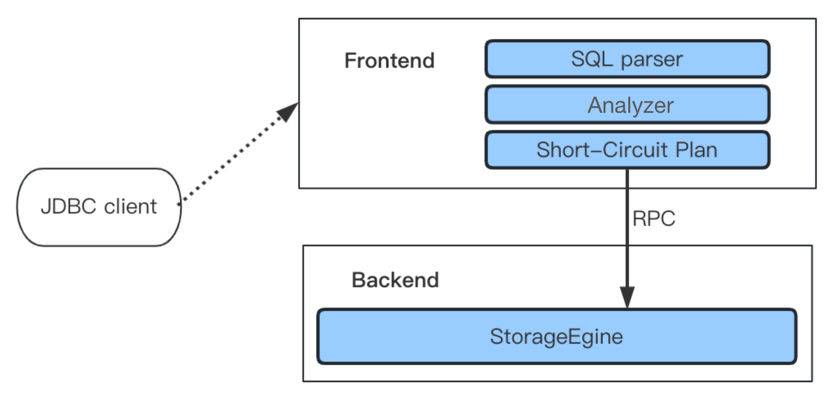
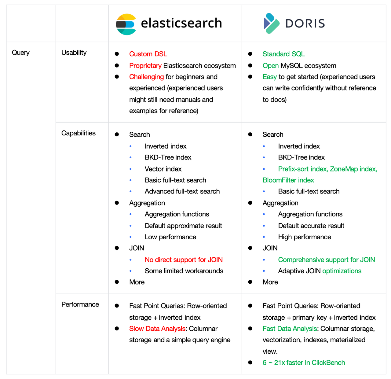
The Doris SQL interface is designed to maintain protocol and syntax compatibility with MySQL. It even does not have its own client or JDBC driver, allowing the use of MySQL’s client and JDBC driver directly. This is a big convenience for many users familiar with MySQL. In fact, this choice was made early in the original design of Doris to make it more user-friendly. Since MySQL is the most widely used open-source OLTP database, Doris is designed to complement MySQL, creating the best practice for combining OLTP (MySQL) with OLAP (Doris). This allows engineers and data analysts to work seamlessly within a single interface and set of syntax, covering both transactional and analytical workloads.

On the other hand, Elasticsearch has its own Domain Specific Language (DSL), which is originally designed for searching. This DSL is part of the Elasticsearch ecosystem, it often requires engineers to invest a lot of time and effort to fully understand and use the DSL effectively.

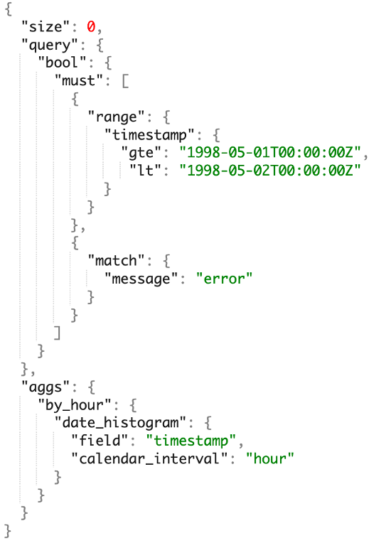
Let's take a look at one example:

Real-time queries.png

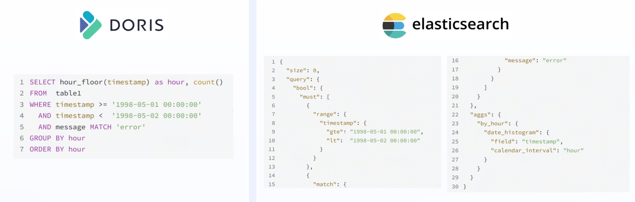
Imagine we want to search for a particular keyword within a particular time range, and then group and order the data by time interval to visualize it as a trend chart.

In Doris, this can be done with only 7 lines of SQL. However, in Elasticsearch, the same process requires 30 lines.

And it's not just about the code complexity. I believe many of you may find this relatable: The first attempt to learn Elasticsearch's DSL is quite challenging. And even after gaining familiarity with it, crafting a query often requires frequent reference to documentation and examples. Due to its inherent complexity, writing DSL queries from scratch remains a challenging task. In contrast, SQL is simple, clear, and highly structured. Most engineers can easily write a query like this without much effort.

Query capabilities

Elasticsearch is good at searching. As its name suggests, it was built for search. But beyond search and aggregation queries, it doesn't support complex analytical queries, such as multi-table JOIN.

Apache Doris is a general-purpose data warehouse. It provides strong support for complex analytics, including multi-table JOIN, UDF, subquery, window function, logic view, materialized view, and data lakehouse. And Doris has been improving its searching capabilities since version 2.0. We have introduced inverted index and full-text search, so it is getting increasingly competitive in this area.

While this article focuses on real-time analytics scenarios, we have chosen not to overlook Elasticsearch’s core strength: its search capabilities.

Elasticsearch, renowned for its search performance, leverages the Apache Lucene library under the hood. It provides two primary indexing structures:

  • Inverted indexes for text fields.
  • BKD-Tree indexes for numeric, date, and geospatial data.

Elasticsearch supports the following search paradigms:

  1. Exact Matching: equality or range queries for numeric, date, or non-tokenized string fields (keyword), powered by BKD-Tree indexes (numeric/date) or non-tokenized inverted indexes (exact term matches).
  2. Full-Text Search: keyword, phrase, or multi-term matching. During ingestion, text is split into tokens using a configurable tokenizer. Queries match tokens, phrases, or combinations (e.g., "quick brown fox"). Elasticsearch supports some advanced full-text search features, such as relevance scoring, auto-completion, spell-checking, and search suggestions.
  3. Vector Search based on ANN index.

Doris also supports a rich set of indexes to accelerate queries, including prefix-sorted indexes, ZoneMap indexes, BloomFilter indexes and N-Gram BloomFilter indexes.

Starting from version 2.0, Doris has added inverted indexes and BKD-Tree indexes to support exact matching and full-text search. Vector search is currently under development and is expected to be available within the next six months.

There are some differences between the indexes of Apache Doris and Elasticsearch:

  1. Diverse indexing strategies: Doris does not rely solely on inverted indexes for query acceleration. It offers different indexes for different scenarios. ZoneMap, BloomFilter, and N-Gram BloomFilter indexes are skip indexes that accelerate analytical queries by skipping non-matching data blocks based on WHERE conditions. The N-Gram BloomFilter index is specifically optimized for LIKE-style fuzzy string matching. Inverted index and Prefix-sorted indexes are point query indexes that speed up point queries by locating which rows satisfy the WHERE conditions through the index and directly read those rows.
  2. Performance centric design: Doris prioritizes speed and efficiency over advanced search features. To achieve faster index building and query performance (see the Query Performance section in the following), it omits certain complex functionalities of inverted indexes at present, such as relevance scoring, auto-completion, spell-checking, and search suggestions. Since there are more critical in document or web search scenarios, which are not Doris’ primary focus on real-time analytics.

For exact matching and common full-text search requirements, such as term, range, phrase, multi-field matching, Doris is fully capable and reliable in most use cases. For complex search needs (e.g., relevance scoring, auto-completion, spell-checking, or search suggestions), Elasticsearch remains the more suitable choice.

Aggregation

Both Elasticsearch and Doris support a wide range of aggregation operators, including:

  • Basic aggregations: MIN, MAX, COUNT, SUM, AVG.
  • Advanced aggregations: PERCENTILE (quantiles), HISTOGRAM (bucketed distributions).
  • Aggregation modes: Global aggregation, key-based grouping (e.g., GROUP BY).

However, their approaches to aggregation analysis differ significantly in the following aspects:

1. Query syntax and usability: Doris uses standard SQL syntax (GROUP BY clauses + aggregation functions), making it intuitive for analysts and developers familiar with SQL. Elasticsearch relies on a custom Domain-Specific Language (DSL) with concepts like metric agg, bucket agg, and pipeline agg. Complexity increases with nested or multi-layered aggregations, requiring steeper learning curves.

2. Result accuracy: Elasticsearch outputs inaccurate approximate result for many aggregation types by default. Aggregations (e.g., terms agg) are executed per shard, with each shard returning only its top results (e.g., top 10 buckets). These partial results are merged globally, leading to potentially inaccurate final outputs. As a serious OLAP database, Doris ensures exact results by processing full datasets without approximations.

3. Query Performance: Doris demonstrates significant performance advantages over Elasticsearch in aggregation-heavy OLAP workloads like those on ClickBench (see more in the Query performance section bellow).

JOIN

Elasticsearch does not support JOIN, making it unable to execute common benchmarks like TPC-H or TPC-DS. Since JOINs are critical in data analysis, Elasticsearch provides some complex workarounds with significant limitations:

  1. Parent-child relationships and has_child / has_parent queries: Simulate JOINs by establishing parent-child relationships within a single index. Child documents store the parent document’s ID. has_child queries first find matching child documents, then retrieve their parent documents via the stored parent IDs. has_parent queries reverse this logic. It's complex and Elasticsearch explicitly warns against equating this approach to database-style JOINs.

    We don’t recommend using multiple levels of relations to replicate a relational model. Each level of relation adds an overhead at query time in terms of memory and computation. For better search performance, denormalize your data instead.

  2. Terms lookup: Similar to an IN-subquery by fetching a value list from one index and using it in a terms query on another. It's only suitable for large-table-to-small-table JOINs (e.g., filtering a large dataset using a small reference list), but performs very poorly for large-table-to-large-table JOINs due to scalability issues.

Doris provides comprehensive support for JOIN operations, including:

  • INNER JOIN
  • CROSS JOIN
  • LEFT / RIGHT / FULL OUTER JOIN
  • LEFT / RIGHT SEMI JOIN
  • LEFT / RIGHT ANTI JOIN

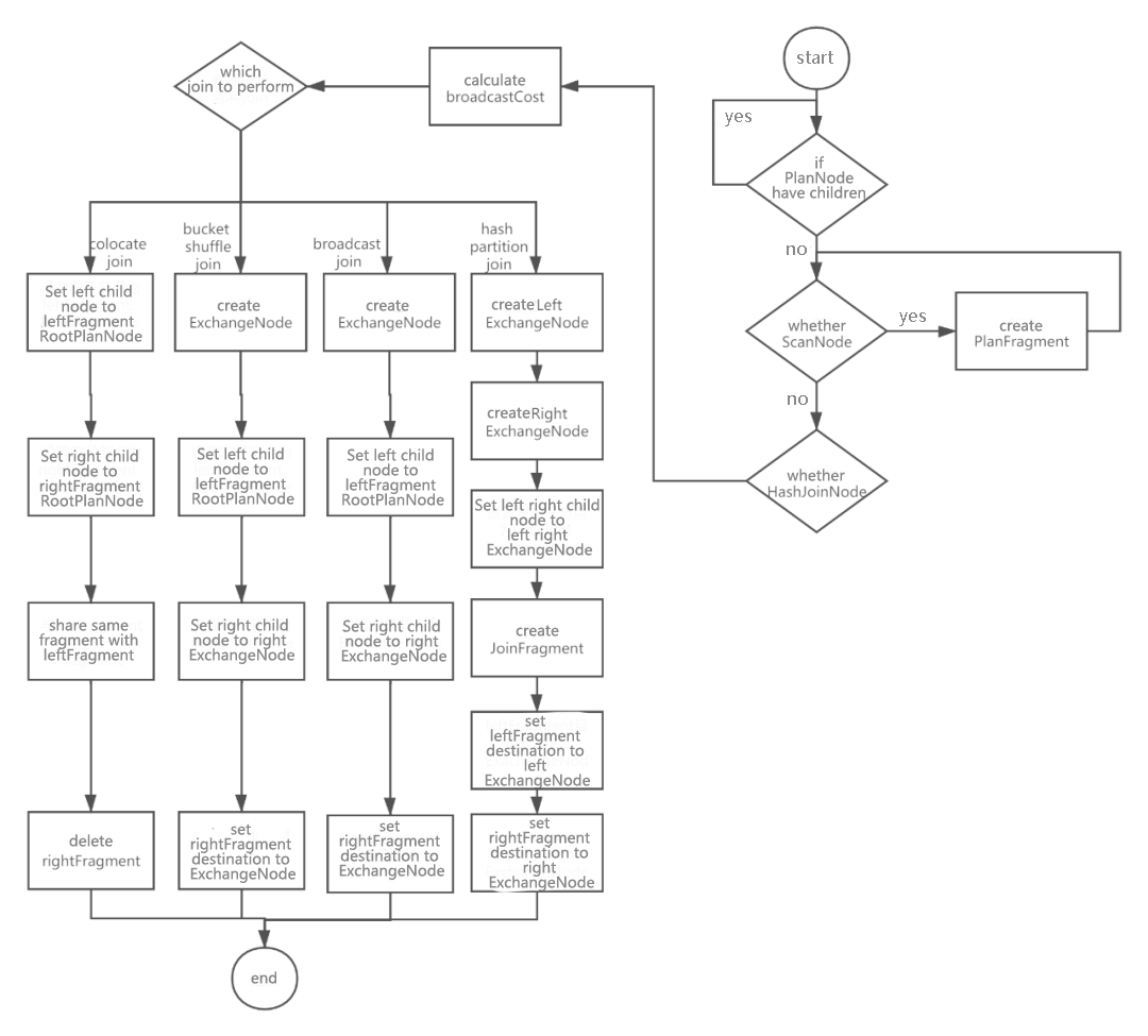
Further more, Doris’ query optimizer adaptively selects optimal execution plans for JOIN operations based on data characteristics and statistics, including:

  • Small-large table JOIN:
    • Broadcast JOIN: The smaller table is broadcast to all nodes for local joins.
  • Large-large table JOIN:
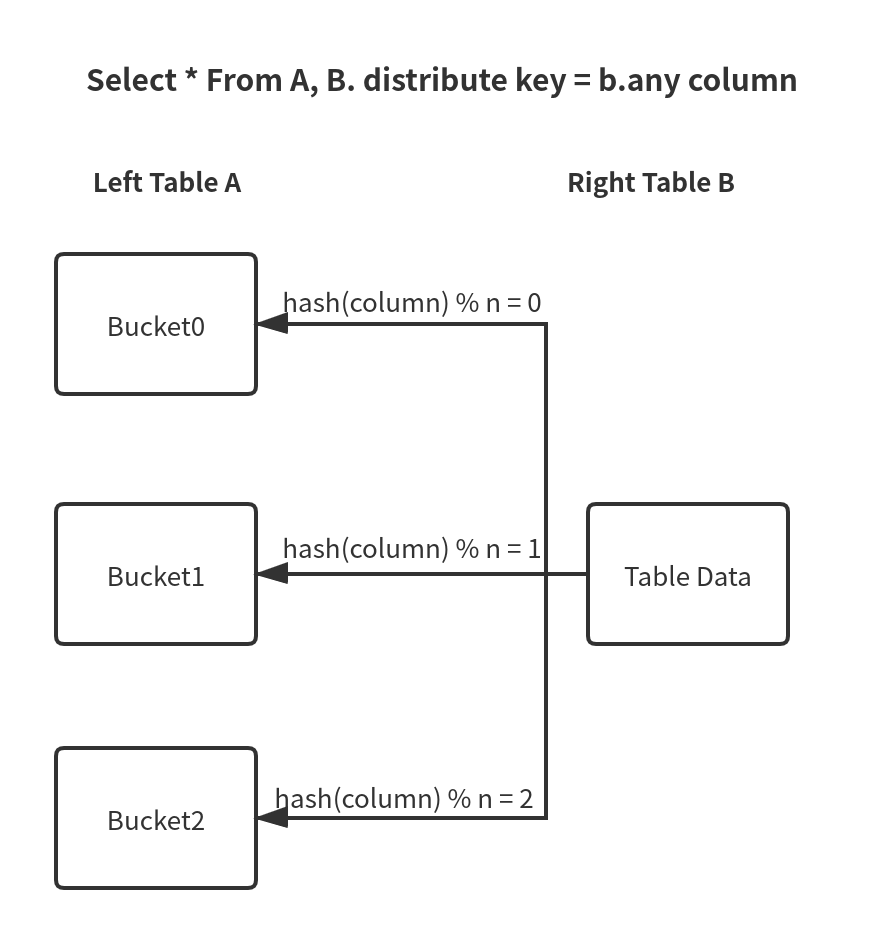
    • Bucket Shuffle JOIN: Used when the left table’s bucketing distribution aligns with the JOIN key.
    • Colocate JOIN: Applied when both the left and right tables share identical bucketing distributions with the JOIN keys.
    • Runtime Filter: Reduces data scanned in the left table by pushing down predicates from the right table using runtime-generated filters.

This intelligent optimization ensures efficient JOIN execution across diverse data scales and distributions, including TPC-H and TPC-DS benchmarks.

Lakehouse

Data warehouses addresses the need for fast data analysis, while data lakes are good at data storage and management. The integration of them, known as "lakehouse", is to facilitate the seamless integration and free flow of data between the data lake and data warehouse. It enables users to leverage the analytic capabilities of the data warehouse while harnessing the data management power of the data lake.

lakehouse.png

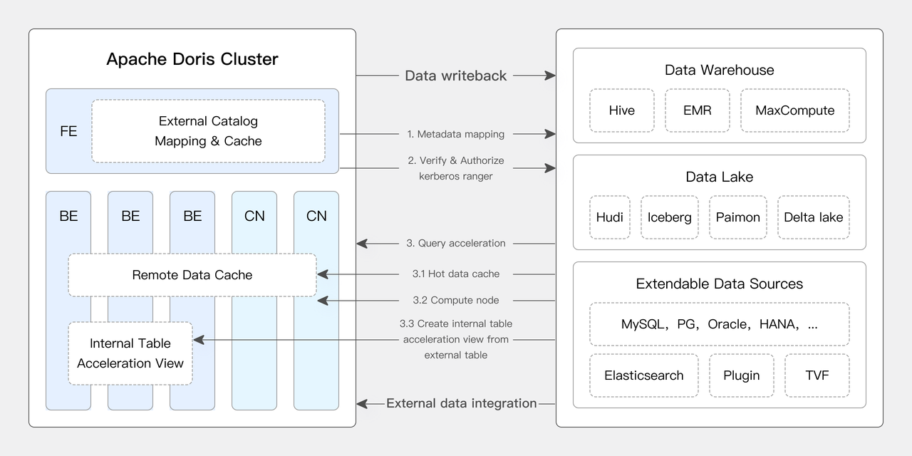
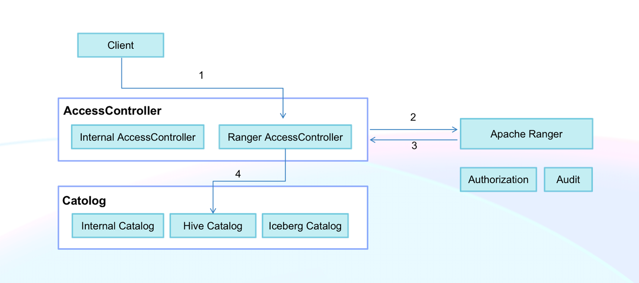
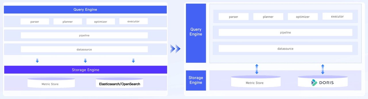
Apache Doris can work as a data lakehouse with its Multi Catalog feature. It can access databases and data lakes including Apache Hive, Apache Iceberg, Apache Hudi, Apache Paimon, LakeSoul, Elasticsearch, MySQL, Oracle, and SQLServer. It also supports Apache Ranger for privilege management.

Elasticsearch does not support querying external data, and of course, it does not support lakehouse either.

Query performance

Apache Doris has been extensively optimized for multiple scenarios, so it can deliver high performance in many use cases. For example, Doris can achieve tens of thousands of QPS for high-concurrency point queries, and it delivers industry-leading performance in aggregation analysis on a global scale.

Elasticsearch is good at point queries (retrieving just a small amount of data). However, it might struggle with complex analytical workloads.

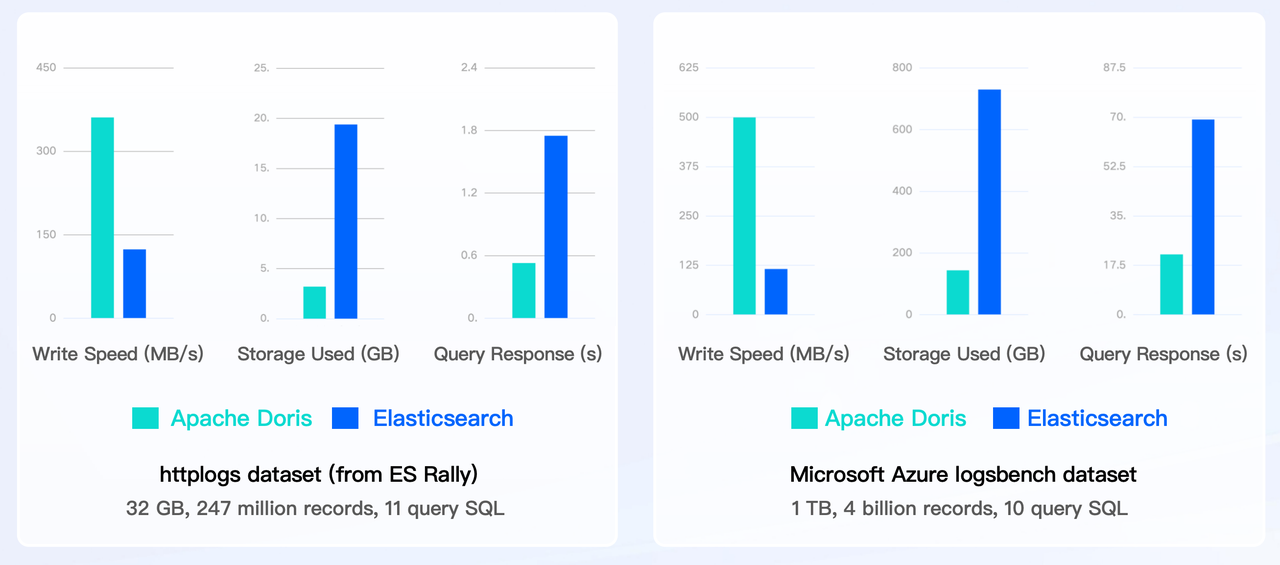
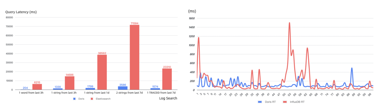
Elasticsearch httplogs and the Microsoft Azure logsbench are benchmarks for log storage and search. Both tests show that Doris is about 34 times faster than Elasticsearch in data writing, but only uses 1/61/4 of the storage space that Elasticsearch uses. Then for data queries, Doris is more than 2 times faster than Elasticsearch.

Query performance.png

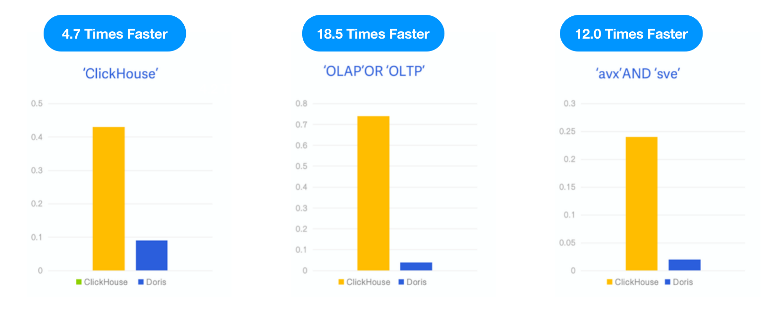
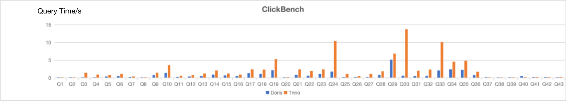
ClickBench is a benchmark created and maintained by the ClickHouse team to evaluate the performance of analytical databases. It results show that Apache Doris delivers out-of-the-box query performance 21 times faster than Elasticsearch and 6 times faster than a fine-tuned Elasticsearch.

Query performance-2.png

Comparison Summary

In summary, Doris follows Apache License 2.0, which is a highly open license to ensure that Doris remains truly open and will continue to uphold such openness in the future.

Secondly, Doris supports both compute-storage coupled and decoupled mode, while Elasticsearch only supports the former, which enable more powerful elasticity and resource isolation.

Thirdly, Doris provides high performance in data ingestion. It is usually 3~5 times faster than Elasticsearch.

In terms of storage, compared to Elasticsearch, Doris can reduce storage costs by 70% or more. It is also 10 times faster than Elasticsearch in data updates.

As for data queries, Doris outperforms Elasticsearch by a lot. It also provides analytic capabilities that Elasticsearch does have, including multi-table JOIN, materialized views, and data lakehouse.

comparisons.png comparisons-2.png comparisons-3.png

Use cases

Many users have replaced Elasticsearch with Apache Doris in their production environments and received exciting results. I will introduce some user stories from the fields of observability, cyber security, and real-time business analysis.

Observability

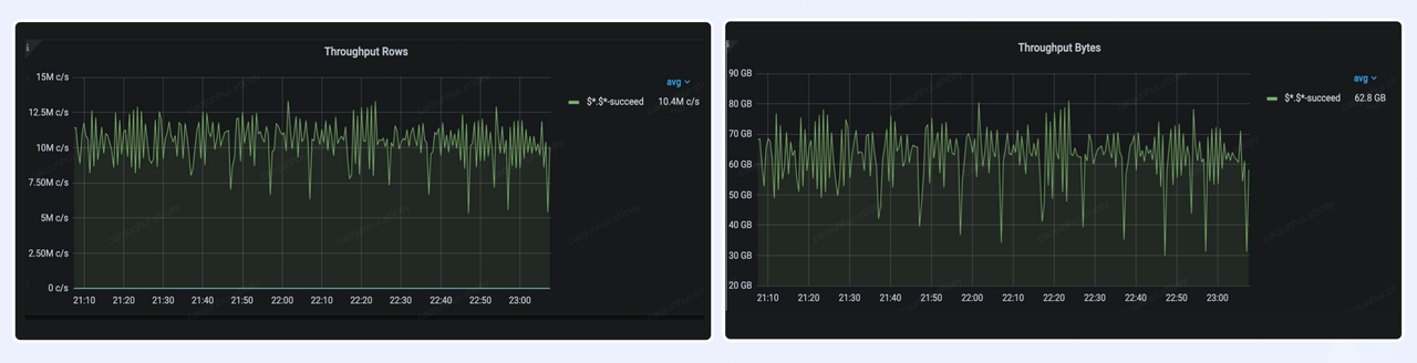
User A: a world-famous short video provider

  • Daily incremental data: 800 billion rows (500 TB)
  • Average write throughput: 10 million row/s (60GB/s)
  • Peak write throughput: 30 million row/s (90GB/s)

Apache Doris supports logging and tracing data storage for this tech giant and meets the data import performance requirements for nearly all use cases within the company.

Observability.png

User B: NetEase - one of the World's Highest-Yielding Game Companies

  • Replacing Elasticsearch with Apache Doris for log analysis: reducing storage consumption by 2/3 and achieving 10X query performance
  • Replacing InfluxDB with Apache Doris for time-series data analysis: saving 50% of server resources and reducing storage consumption by 67%

Observability-2.png

User C: an observability platform provider

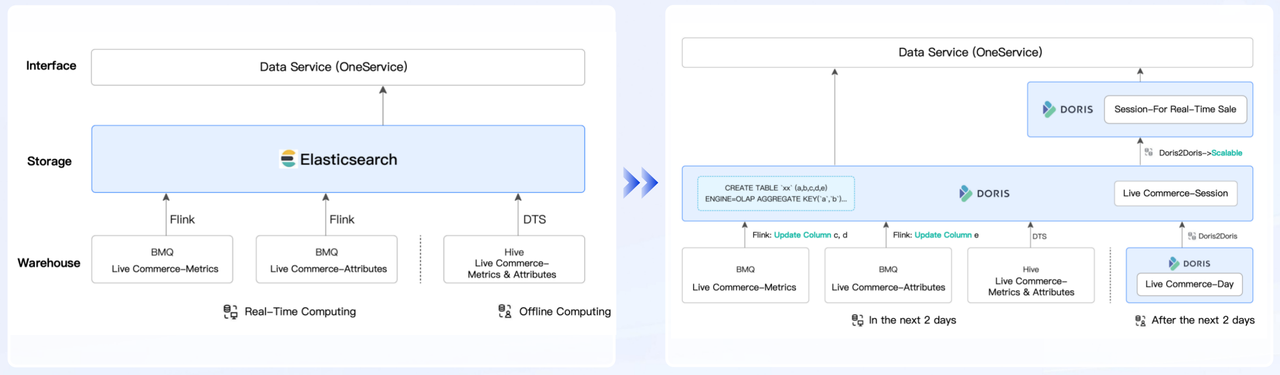
Apache Doris offers a special data type, VARIANT, to handle semi-structured data in log and tracing, reducing costs by 70% and delivering 2~3 times faster full-text search performance compared to the Elasticsearch-based solution.

Observability-3.png

Cyber security

User A: QAX - a listed company & leading cyber security leader

The Doris-based security logging solution uses 40% less storage space, delivers 2X faster write performance, and supports full-text search, aggregation analysis, and multi-table JOIN capabilities in one database system.

Cyber security.png

User B: a payment platform with nearly 600 million registered users

As a unified security data storage solution, Apache Doris delivers 4X faster write speeds, 3X better query performance, and saves 50% storage space compared to the previous architecture with diverse tech stacks using Elasticsearch, Hive and Presto.

Cyber security-2.png

User C: a leading cyber security solution provider

Compared to Elasticsearch, Doris delivers 2 times faster write speeds, 4 times better query performance, and a 4 times data compression ratio.

Cyber security-3.png

Business analysis

User A: a world-leading live e-commerce company

The user previously relied on Elasticsearch to handle online queries for their live stream detail pages, but they faced big challenges in cost and concurrency. After migrating to Apache Doris, they achieve:

  • 3 times faster real-time writes: 30w/s -> 100w/s
  • 4 times higher query concurrency: 500QPS -> 2000QPS

Business analysis.png

User B: Tencent Music Entertainment

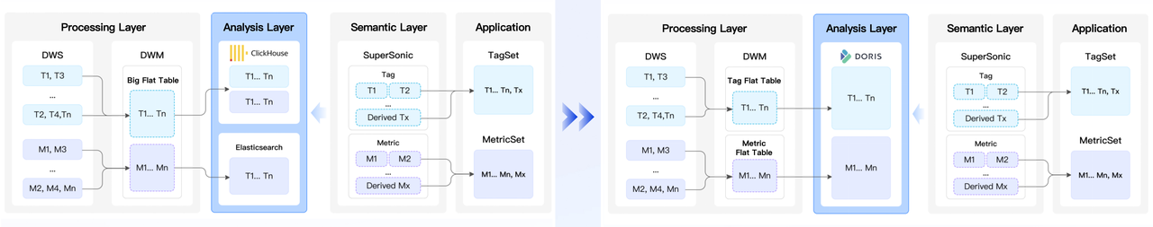
Previously, TME content library used both Elasticsearch and ClickHouse to meet their needs for data searching and analysis, but managing two separate systems was complex and inefficient. With Doris, they are able to unify the two systems into one single platform to support both data searching and analysis. The new architecture delivers 4X faster write speeds, reduces storage costs by 80%, and supports complex analytical operations.

Business analysis-2.png

User C: a web browser provider with 600 million users

After migrating to Apache Doris for a unified solution for log storage and report analysis, the company doubled its aggregation analysis efficiency, reduced storage consumption by 60%, and cut SQL development time by half.

Business analysis-3.png

Taking Apache Doris to the next level

Taking Apache Doris to the next level.png

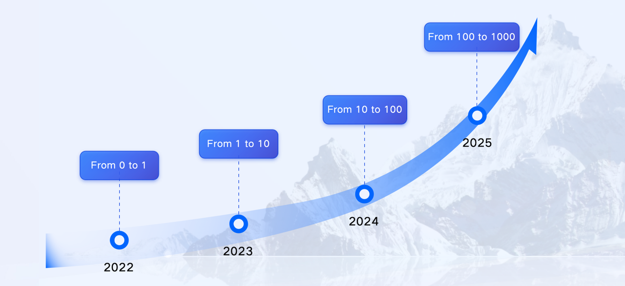
For the Apache Doris community developers, the path to making Doris good enough to replace Elasticsearch wasn't easy. In 2022, we started adding inverted index capabilities to Doris. At that time, this decision was met with skepticism. Many viewed inverted indexes as a feature exclusive to Elasticsearch, a domain few in the industry dared to venture into. Nevertheless, we went with it, and today we can confidently say that we have succeeded.

In 2022, we developed this feature from the ground up, and after a year of dedicated effort, we open-sourced it. Initially, we had only one user, QAX, who was willing to test and adopt the feature. We are deeply grateful to them for their early support during this pivotal stage.

By 2023, the value of Doris with inverted indexes became increasingly evident, leading to broader adoption by about 10 companies.

The growth momentum has continued, and as of 2024, we are experiencing rapid expansion, with over 100 companies now leveraging Doris to replace Elasticsearch.

Looking ahead, I am very much looking forward to what 2025 will bring. This progress, advancing from the ground up to such significant milestones, has been made possible by the incredible support from the Doris community users and developers. We encourage everyone to join the Apache Doris Slack community and join the dedicated channel #elasticsearch-to-doris, where you can receive technical assistance, stay updated with the latest news about Doris, and engage with more Doris developers and users.

More on Apache Doris:

Connect with me on Linkedin

Apache Doris on GitHub

Apache Doris Website

Blog/Tech Sharing

Apache Doris

In the age of data-driven decision-making, the exponential growth of data volume and the ever-evolving demands for analytics pose great challenges. Data streams in from diverse sources (such as application logs, network interactions, and mobile devices), spanning structured, semi-structured, and unstructured formats. This diversity places pressure on storage and analytical systems. Meanwhile, the surge in demand for real-time analytics and exploratory queries requires systems to deliver millisecond-level responsiveness while achieving optimal cost efficiency and elastic scalability.

Apache Doris emerged in the era of integrated storage and computation, built on a classic Shared Nothing architecture. In this design, storage and computation are co-located on Backend (BE) nodes, leveraging an MPP (Massively Parallel Processing) distributed computing model. This architecture delivers key advantages, including high availability, simplified deployment, seamless horizontal scalability, and exceptional real-time analytical performance.

For real-time analytics and small-scale data processing, Apache Doris stands out with predictable, stable low-latency performance, making it an indispensable solution. However, when scaling to large-scale data processing, it encounters certain challenges, primarily in:

  • Relatively high costs & low elasticity: Balancing storage and compute resources remains a big challenge. Storage capacity must be sufficient to accommodate all data, while compute resources need to handle query workloads efficiently. However, dynamically scaling clusters is often time-consuming, prompting enterprises to over-provision resources to ensure stability. This approach simplifies operations but leads to resource waste and increased costs.
  • Limited workload isolation: Since Apache Doris 2.0, Workload Groups provide soft isolation, while Resource Groups offer a degree of hard isolation. However, neither mechanism ensures complete physical isolation, which can impact performance in multi-tenant or resource-intensive environments.
  • Operational complexity: Managing an OLAP system with built-in distributed storage requires not only overseeing compute nodes but also ensuring efficient storage administration. Storage management is inherently complex, and misconfigurations or improper operations can lead to data loss, making maintenance highly demanding.

Even so, in the absence of stable and large-scale storage support, a integrated storage-compute architecture remains the optimal choice.

As cloud infrastructure matures, enterprises increasingly seek deeper Apache Doris integration with public clouds, private clouds, and Kubernetes (K8s) container platforms to unlock greater elasticity and flexibility. Public clouds offer mature object storage with on-demand compute resources, eliminating the need for pre-allocated space, while private clouds leverage technologies like K8s and MinIO to build scalable resource platforms. This evolution in cloud infrastructure has also accelerated Apache Doris’ transition to a storage-compute decoupled architecture, enabling lower costs, high elasticity, and enhanced workload isolation.

Apache Doris Compute-Storage Decoupled Mode

Since version 3.0, Apache Doris has supported both the compute-storage decoupled mode and the compute-storage coupled mode.

01 Compute-Storage Decoupled

In the compute-storage decoupled mode, Apache Doris adopts a three-tier architecture consisting of three layers: shared storage, compute groups, and meta data service:

compute-storage-decoupled.jpg

Shared Storage Layer

Data is persisted in the shared storage layer, allowing compute nodes to access and share data seamlessly. This design enhances compute node flexibility and reduces operational overhead. Leveraging mature and reliable shared storage results in ultra-low storage costs and high data reliability. Whether using public cloud object storage or enterprise-managed shared storage, this approach greatly reduces the maintenance complexity of Apache Doris.

Compute Groups

The compute layer consists of multiple compute groups responsible for executing query plans. Each query is executed within a single compute group, ensuring isolation and scalability. Compute nodes are stateless, utilizing local disks as high-speed caches to accelerate queries while sharing the same data and metadata services. Each compute group operates independently, supporting on-demand scaling, and local caches remain isolated to ensure workload separation and performance consistency.

Meta Data Service

The meta data layer manages system meta data, including databases, tables, schemas, rowset meta data, and transaction information, with support for horizontal scaling. Future iterations of Apache Doris’ compute-storage decoupled mode will introduce stateless Frontend (FE) nodes, where memory consumption is decoupled from cluster size. This evolution will eliminate memory bottlenecks, allowing FE nodes to operate with minimal memory requirements.

02 Architecture Design

Traditional compute-storage decoupling approaches typically store both data and meta data in shared storage while centralizing transaction management on a single FE node. However, this design introduces several challenges:

  • Write performance bottlenecks: The two-phase commit protocol, driven by FE Master, incurs high latency and low throughput.
  • Small file proliferation: Frequent meta data writes generate excessive small files, leading to system instability and inflated storage costs.
  • Scalability constraints: Since FE nodes manage meta data in memory, an increasing number of Tablets amplifies memory pressure, eventually causing write bottlenecks.
  • Data deletion risks: Relying on delta computation with timeout-based mechanisms for deletion introduces challenges in synchronizing writes and deletions. As a result, there is a risk of unintended data loss due to misalignment between ongoing writes and scheduled deletions.

Compared to traditional approaches, Apache Doris effectively addresses these challenges through a shared meta data service:

  • Real-time ingestion: The meta data service provides a globally consistent view, enabling low-latency, high-throughput writes. Benchmarks show that the Apache Doris compute-storage decoupled mode achieves 100X higher performance than other solutions at 50 concurrent writes and 11X higher performance at 500 concurrent writes.
  • Optimized small file management: Data is written to shared storage, while meta data is handled by the meta data service. This effectively reduces small file overheads. Tests indicate that the Apache Doris compute-storage decoupled mode generates only 1/2 the number of write files compared to other industry solutions.
  • Enhanced scalability: In future versions of Apache Doris, FE metadata will be moved to the meta data service to eliminate cluster scaling limitations and ensure seamless expansion.
  • Reliable data deletion: Doris employs a forward deletion mechanism based on a globally consistent view. This ensures mutual exclusion between writes and deletions, thus eliminating the risk of accidental data loss.

03 What makes it stand out

The Apache Doris compute-storage decoupled architecture provide values for users in three aspects: cost efficiency, elasticity, and workload isolation.

Firstly, it brings a 90% cost reduction compared to the compute-storage coupled mode.

  • Pay-as-you-go: Unlike traditional coupled architectures, there’s no need to pre-provision compute and storage resources. Storage costs scale with actual usage, while compute resources can be dynamically adjusted based on demand.
  • Single-replica storage: Instead of maintaining three replicas in costly block storage, data is stored as a single replica in low-cost object storage, with hot data cached in block storage for performance. This dramatically reduces storage footprint and hardware costs. For example, S3 costs only 25% to 50% of AWS EBS.
  • Lower resource consumption: In compute-storage decoupled mode, compaction operations only process a single data replica, thus largely reducing resource usage compared to multi-replica environments.

Secondly, with a stateless compute node design, Doris enables on-demand resource scaling to meet fluctuating workloads efficiently.

  • Elastic auto-scaling: Compute resources can be dynamically scaled to accommodate traffic spikes or workload variations. When demand increases, Doris can rapidly scale out compute nodes; when demand drops, resources scale down automatically, avoiding unnecessary costs.
  • Fine-grained compute resource allocation: Doris allows compute nodes to be strategically assigned to specific compute groups based on workload requirements. For example, high-performance nodes handle complex queries and high-concurrency workloads, while standard nodes manage lightweight queries and infrequent requests.

Thirdly, Doris provides efficient resource scheduling and workload isolation mechanisms.

  • Cross-business isolation: Different business units can be assigned dedicated compute groups with physical isolation, so workloads operate on dedicated resources without interference.
  • Offline workload isolation: Large-scale batch processing tasks can be segregated into dedicated compute groups, so users can leverage low-cost resources for offline data processing without impacting real-time business performance.
  • Read-write isolation: Doris allows dedicated compute groups for read and write operations to ensure consistent query response times even under high write loads.

Benchmarking and comparison

To provide a clear evaluation of the compute-storage decoupled architecture of Apache Doris, we conducted a series of benchmark tests across multiple dimensions, including data ingestion, query performance, and resource cost efficiency.

01 Ingestion performance

High-concurrency ingestion

We compared Apache Doris' coupled and decoupled modes with other mainstream solutions under the same compute resources. The tests measured real-time ingestion performance under two levels of concurrency:

  • 50 concurrent writes: Ingesting 250 files, each containing 20,000 rows.
  • 500 concurrent writes: Ingesting 10,000 files, each containing 500 rows.

Test results:

  • At 50 concurrent writes, Doris' compute-storage decoupled mode performed on par with the coupled mode while achieving 100X the write performance of other industry compute-storage decoupled solutions.
  • At 500 concurrent writes, Doris' decoupled mode experienced a slight performance drop compared to the coupled mode, yet still maintained an 11X advantage over other compute-storage decoupled architectures.

high-concurrency-ingestion.jpg

Batch data ingestion

To evaluate batch data ingestion efficiency, we conducted tests using TPC-H 1TB and TPC-DS 1TB datasets, comparing the compute-storage coupled and decoupled modes of Apache Doris. Data was loaded using S3 Load. Under default configurations, multiple tables were ingested sequentially, and the total ingestion time was measured for comparison.

Hardware configuration:

  • Cluster size: 4 compute instances (1 FE, 3 BE)
  • CPU: 48 cores per instance
  • Memory: 192GB per instance
  • Network Bandwidth: 21 Gbps
  • Storage: Enhanced SSD

batch-data-ingestion.jpg

As is shown, even when using a single replica in both architectures, the compute-storage decoupled mode outperforms the coupled mode in batch data ingestion by 20.05% and 27.98% in the two benchmarks, respectively. (In real-world deployments, the coupled mode typically adopts a three-replica strategy. This further amplifies the write performance gains of the decoupled mode.)

02 Query Performance

In the compute-storage decoupled mode, Apache Doris leverages a multi-tier caching mechanism to accelerate queries. It improves overall query efficiency by speeding up data access and minimizing reliance on shared storage. The cache hierarchy includes:

  • Doris Page Cache: In-memory caching of decompressed data.
  • Linux Page Cache: In-memory caching of compressed data.
  • Local Disk Cache: Persistent caching of compressed data.

Hardware configuration:

  • Cluster size: 4 compute instances (1 FE, 3 BE)
  • CPU: 48 cores per instance
  • Memory: 192GB per instance
  • Network Bandwidth: 21 Gbps
  • Storage: Enhanced SSD

We conducted performance benchmarking under different caching scenarios in both compute-storage coupled and decoupled modes. Using the TPC-DS 1TB dataset, the test results are as follows:

query-performance.jpg

  • Full cache hit: We execute the query twice and measure the runtime of the second execution, ensuring that all data is preloaded into the cache. Query performance in compute-storage decoupled mode matches that of the coupled architecture with no performance degradation.
  • Partial cache hit (This scenario best reflects real-world usage.): Before the test begins, all caches are cleared, and we measure the runtime of the first execution while data is gradually loaded into the cache. Compared to the coupled architecture, query performance remains nearly identical, with an overall performance overhead of about 10%.
  • No cache hit: All caches are cleared before each SQL execution, ensuring that every query runs without cached data. Compared to the coupled architecture, query performance sees an approximate 35% degradation.

03 Resource Cost

Operational cost for online workloads

Taking a real-world enterprise workload as an example, we compare the cost differences between compute-storage coupled and decoupled modes in Apache Doris.

  • Compute-storage coupled mode: The dataset in Doris has a size of 100TB per replica, resulting in a total of 300TB with three replicas. To prevent frequent scaling operations from impacting business stability, disk usage is maintained at about 50%. Thus, the monthly resource cost amounts to $36,962.7 (as detailed below).

operational-cost-for-online-workloads.jpg

  • Compute-storage decoupled mode: With the same data scale, adopting the compute-storage decoupled model only requires storing a single replica in object storage, while hot data is cached on local disks. As shown below, the monthly resource cost is reduced to $22,212.65, achieving a 40% cost savings.

compute-storage-decoupled-mode.jpg

Historical data cost

For example, with 200TB of historical data, the resource utilization under both the compute-storage coupled and decoupled modes is shown below. The coupled model incurs a monthly cost of $48,851.10, whereas the decoupled model reduces the cost to just $4,502.40—cutting expenses by over 90%.

historical-data-cost.jpg

What's next

Powered by compute-storage decoupling, Apache Doris excels in real-time analytics, lakehouse analytics, observability and log storage & analysis. Looking ahead, Apache Doris will continue to enhance its capabilities in this mode. We will introduce new features such as snapshots, time travel, and Cross-Cluster Replication (CCR) support, and achieve stateless FE to further improve system stability and usability.

If you're interested in Apache Doris' compute-storage decoupled mode and its future development, we invite you to join the #compute-storage-decoupled channel in the Apache Doris Slack community, where you can connect with core developers and users. We look forward to your thoughts and contributions!

Join us live on March 27 for more insights into the Apache Doris compute-storage decoupled mode!

Blog/Tech Sharing

Apache Doris

To handle large datasets, distributed databases introduce strategies like partitioning and bucketing. Data is divided into smaller units based on specific rules and distributed across different nodes, so databases can perform parallel processing for higher performance and data management flexibility.

Like in many databases, Apache Doris shards data into partitions, and then a partition is further divided into buckets. Partitions are typically defined by time or other continuous values. This allows query engines to quickly locate the target data during queries by pruning irrelevant data ranges.

Bucketing, on the other hand, distributes data based on the hash values of one or more columns, which prevents data skew.

Prior to version 2.1.0, there are two way you can create data partitions in Apache Doris:

  • Manual Partition: Users specify the partitions in the table creation statement, or modify them through DDL statements afterwards.

  • Dynamic Partition: The system automatically maintains partitions within a pre-defined range based on the data ingestion time.

In Apache Doris 2.1.0, we have introduced Auto Partition. It supports partitioning data by RANGE or by LIST and further enhances flexibility on top of automatic partitioning.

Evolution of partitioning strategies in Doris

In the design of data distribution, we focus more on partition planning, because the choice of partition columns and partition intervals heavily depends on the actual data distribution patterns, and a good partition design can largely improve the query and storage efficiency of the table.

In Doris, the data table is divided into partitions and then buckets in a hierarchical manner. The data within the same bucket then forms a data tablet, which is the minimum physical storage unit in Doris for data replication, inter-cluster data scheduling, and load balancing.

Evolution of partitioning strategies in Doris

Manual Partition

Doris allows users to manually create data partitions by RANGE and by LIST.

For time-stamped data like logs and transaction records, users typically create partitions based on the time dimension. Here's an example of the CREATE TABLE statement:

CREATE TABLE IF NOT EXISTS example_range_tbl
(
`user_id` LARGEINT NOT NULL COMMENT "User ID",
`date` DATE NOT NULL COMMENT "Data import date",
`timestamp` DATETIME NOT NULL COMMENT "Data import timestamp",
`city` VARCHAR(20) COMMENT "Location of user",
`age` SMALLINT COMMENT "Age of user",
`sex` TINYINT COMMENT "Sex of user",
`last_visit_date` DATETIME REPLACE DEFAULT "1970-01-01 00:00:00" COMMENT "Last visit date of user",
`cost` BIGINT SUM DEFAULT "0" COMMENT "User consumption",
`max_dwell_time` INT MAX DEFAULT "0" COMMENT "Maximum dwell time of user",
`min_dwell_time` INT MIN DEFAULT "99999" COMMENT "Minimum dwell time of user"
)
ENGINE=OLAP
AGGREGATE KEY(`user_id`, `date`, `timestamp`, `city`, `age`, `sex`)
PARTITION BY RANGE(`date`)
(
PARTITION `p201701` VALUES LESS THAN ("2017-02-01"),
PARTITION `p201702` VALUES LESS THAN ("2017-03-01"),
PARTITION `p201703` VALUES LESS THAN ("2017-04-01"),
PARTITION `p2018` VALUES [("2018-01-01"), ("2019-01-01"))
)
DISTRIBUTED BY HASH(`user_id`) BUCKETS 16
PROPERTIES
(
"replication_num" = "1"
);

The table is partitioned by the data import date date, and 4 partitions have been pre-created. Within each partition, the data is further divided into 16 buckets based on the hash value of the user_id.

With this partitioning and bucketing design, when querying data from 2018 onwards, the system only need to scan the p2018 partition. This is what the query SQL looks like:

mysql> desc select count() from example_range_tbl where date >= '20180101';
+--------------------------------------------------------------------------------------+
| Explain String(Nereids Planner) |
+--------------------------------------------------------------------------------------+
| PLAN FRAGMENT 0 |
| OUTPUT EXPRS: |
| count(*)[#11] |
| PARTITION: UNPARTITIONED |
| |
| ...... |
| |
| 0:VOlapScanNode(193) |
| TABLE: test.example_range_tbl(example_range_tbl), PREAGGREGATION: OFF. |
| PREDICATES: (date[#1] >= '2018-01-01') |
| partitions=1/4 (p2018), tablets=16/16, tabletList=561490,561492,561494 ... |
| cardinality=0, avgRowSize=0.0, numNodes=1 |
| pushAggOp=NONE |
| |
+--------------------------------------------------------------------------------------+

If the data is distributed unevenly across partitions, the hash-based bucketing mechanism can further divide the data based on the user_id. This helps to avoid load imbalance on some machines during querying and storage.

However, in real-world business scenarios, one cluster may have tens of thousands of tables, which means it is impossible to manage them manually.

CREATE TABLE `DAILY_TRADE_VALUE`
(
`TRADE_DATE` datev2 NOT NULL COMMENT 'Trade date',
`TRADE_ID` varchar(40) NOT NULL COMMENT 'Trade ID',
......
)
UNIQUE KEY(`TRADE_DATE`, `TRADE_ID`)
PARTITION BY RANGE(`TRADE_DATE`)
(
PARTITION p_200001 VALUES [('2000-01-01'), ('2000-02-01')),
PARTITION p_200002 VALUES [('2000-02-01'), ('2000-03-01')),
PARTITION p_200003 VALUES [('2000-03-01'), ('2000-04-01')),
PARTITION p_200004 VALUES [('2000-04-01'), ('2000-05-01')),
PARTITION p_200005 VALUES [('2000-05-01'), ('2000-06-01')),
PARTITION p_200006 VALUES [('2000-06-01'), ('2000-07-01')),
PARTITION p_200007 VALUES [('2000-07-01'), ('2000-08-01')),
PARTITION p_200008 VALUES [('2000-08-01'), ('2000-09-01')),
PARTITION p_200009 VALUES [('2000-09-01'), ('2000-10-01')),
PARTITION p_200010 VALUES [('2000-10-01'), ('2000-11-01')),
PARTITION p_200011 VALUES [('2000-11-01'), ('2000-12-01')),
PARTITION p_200012 VALUES [('2000-12-01'), ('2001-01-01')),
PARTITION p_200101 VALUES [('2001-01-01'), ('2001-02-01')),
......
)
DISTRIBUTED BY HASH(`TRADE_DATE`) BUCKETS 10
PROPERTIES (
......
);

In the above example, data is partitioned on a monthly basis. This requires the database administrator (DBA) to manually add a new partition each month and maintain table schema regularly. Imagine the case of real-time data processing, where you might need to create partitions daily or even hourly, manually doing this is no long a choice. That's why we introduced Dynamic Partition.

Dynamic Partition

By Dynamic Partition, Doris automatically creates and reclaims data partitions as long as the user specifies the partition unit, the number of historical partitions, and the number of future partitions. This functionality relies on a fixed thread on the Doris Frontend. It continuously polls and checks for new partitions to be created or old partitions to be reclaimed, and updates the partition schema of the table.

This is an example CREATE TABLE statement for a table which is partitioned by day. The start and end parameters are set to -7 and 3, respectively, meaning that data partitions for the next 3 days will be pre-created and the historical partitions that are older than 7 days will be reclaimed.

CREATE TABLE `DAILY_TRADE_VALUE`
(
`TRADE_DATE` datev2 NOT NULL COMMENT 'Trade date',
`TRADE_ID` varchar(40) NOT NULL COMMENT 'Trade ID',
......
)
UNIQUE KEY(`TRADE_DATE`, `TRADE_ID`)
PARTITION BY RANGE(`TRADE_DATE`) ()
DISTRIBUTED BY HASH(`TRADE_DATE`) BUCKETS 10
PROPERTIES (
"dynamic_partition.enable" = "true",
"dynamic_partition.time_unit" = "DAY",
"dynamic_partition.start" = "-7",
"dynamic_partition.end" = "3",
"dynamic_partition.prefix" = "p",
"dynamic_partition.buckets" = "10"
);

Over time, the table will always maintain partitions within the range of [current date - 7, current date + 3]. Dynamic Partition is particularly useful for real-time data ingestion scenarios, such as when the ODS (Operational Data Store) layer directly receives data from external sources like Kafka.

The start and end parameters define a fixed range for the partitions, allowing the user to manage the partitions only within this range. However, if the user needs to include more historical data, they would have to dial up the start value, and that could lead to unnecessary metadata overhead in the cluster.

Therefore, when applying Dynamic Partition, there is a trade-off between the convenience and efficiency of metadata management.

Developers' words

As the complexity of business adds up, Dynamic Partition becomes inadequate because:

  • It only supports partitioning by RANGE but not by LIST.

  • It can only be applied to the current real-world timestamps.

  • It only supports a single continuous partition range, and cannot accommodate partitions outside of that range.

Given these functional limitations, we started to plan a new partitioning mechanism that can both automate partition management and simplify data table maintenance.

We figured out that the ideal partitioning implementation should:

  • Save the need for manually creating partitions after table creation;

  • Be able to accommodate all ingested data in corresponding partitions.

The former stands for automation and the latter for flexibility. The essence of realizing them both is associating partition creation with the actual data.

Then we started to think about: What if we hold off the creation of partitions until the data is ingested, rather than doing it during table creation or through regular polling. Instead of pre-constructing the partition distribution, we can define the "data-to-partition" mapping rules, so the partitions are created after data arrives.

Compared to Manual Partition, this whole process would be fully automated, eliminating the need for human maintenance. Compared to Dynamic Partition, it avoids having partitions that are not used, or partitions that are needed but not present.

Auto Partition

With Apache Doris 2.1.0, we bring the above plan into fruition. During data ingestion, Doris creates data partitions based on the configured rules. The Doris Backend nodes that are responsible for data processing and distribution will attempt to find the appropriate partition for each row of data in the DataSink operator of the execution plan. It no longer filters out data that does not fit into any existing partition or reports an error for such a situation, but automatically generates partitions for all ingested data.

Auto Partition by RANGE

Auto Partition by RANGE provides an optimized partitioning solution based on the time dimension. It is more flexible than Dynamic Partition in terms of parameter configuration. The syntax for it is as follows:

AUTO PARTITION BY RANGE (FUNC_CALL_EXPR)
()
FUNC_CALL_EXPR ::= DATE_TRUNC ( <partition_column>, '<interval>' )

The <partition_column> above is the partition column (i.e., the column that the partitioning is based on). <interval>specifies the partition unit, which is the desired width of each partition.

For example, if the partition column is k0 and you want to partition by month, the partition statement would be AUTO PARTITION BY RANGE (DATE_TRUNC(k0, 'month')). For all the imported data, the system will call DATE_TRUNC(k0, 'month') to calculate the left endpoint of the partition, and then the right endpoint by adding one interval.

Now, we can apply Auto Partition to the DAILY_TRADE_VALUE table introduced in the previous section on Dynamic Partition.

CREATE TABLE DAILY_TRADE_VALUE
(
`TRADE_DATE` DATEV2 NOT NULL COMMENT 'Trade Date',
`TRADE_ID` VARCHAR(40) NOT NULL COMMENT 'Trade ID',
......
)
AUTO PARTITION BY RANGE (DATE_TRUNC(`TRADE_DATE`, 'month'))
()
DISTRIBUTED BY HASH(`TRADE_DATE`) BUCKETS 10
PROPERTIES
(
......
);

After importing some data, these are the partitions we get:

mysql> show partitions from DAILY_TRADE_VALUE;
Empty set (0.10 sec)

mysql> insert into DAILY_TRADE_VALUE values ('2015-01-01', 1), ('2020-01-01', 2), ('2024-03-05', 10000), ('2024-03-06', 10001);
Query OK, 4 rows affected (0.24 sec)
{'label':'label_2a7353a3f991400e_ae731988fa2bc568', 'status':'VISIBLE', 'txnId':'85097'}

mysql> show partitions from DAILY_TRADE_VALUE;
+-------------+-----------------+----------------+---------------------+--------+--------------+--------------------------------------------------------------------------------+-----------------+---------+----------------+---------------+---------------------+---------------------+--------------------------+----------+------------+-------------------------+-----------+--------------------+--------------+
| PartitionId | PartitionName | VisibleVersion | VisibleVersionTime | State | PartitionKey | Range | DistributionKey | Buckets | ReplicationNum | StorageMedium | CooldownTime | RemoteStoragePolicy | LastConsistencyCheckTime | DataSize | IsInMemory | ReplicaAllocation | IsMutable | SyncWithBaseTables | UnsyncTables |
+-------------+-----------------+----------------+---------------------+--------+--------------+--------------------------------------------------------------------------------+-----------------+---------+----------------+---------------+---------------------+---------------------+--------------------------+----------+------------+-------------------------+-----------+--------------------+--------------+
| 588395 | p20150101000000 | 2 | 2024-06-01 19:02:40 | NORMAL | TRADE_DATE | [types: [DATEV2]; keys: [2015-01-01]; ..types: [DATEV2]; keys: [2015-02-01]; ) | TRADE_DATE | 10 | 1 | HDD | 9999-12-31 23:59:59 | | NULL | 0.000 | false | tag.location.default: 1 | true | true | NULL |
| 588437 | p20200101000000 | 2 | 2024-06-01 19:02:40 | NORMAL | TRADE_DATE | [types: [DATEV2]; keys: [2020-01-01]; ..types: [DATEV2]; keys: [2020-02-01]; ) | TRADE_DATE | 10 | 1 | HDD | 9999-12-31 23:59:59 | | NULL | 0.000 | false | tag.location.default: 1 | true | true | NULL |
| 588416 | p20240301000000 | 2 | 2024-06-01 19:02:40 | NORMAL | TRADE_DATE | [types: [DATEV2]; keys: [2024-03-01]; ..types: [DATEV2]; keys: [2024-04-01]; ) | TRADE_DATE | 10 | 1 | HDD | 9999-12-31 23:59:59 | | NULL | 0.000 | false | tag.location.default: 1 | true | true | NULL |
+-------------+-----------------+----------------+---------------------+--------+--------------+--------------------------------------------------------------------------------+-----------------+---------+----------------+---------------+---------------------+---------------------+--------------------------+----------+------------+-------------------------+-----------+--------------------+--------------+
3 rows in set (0.09 sec)

As is shown, partitions are automatically created for the imported data, and it doesn't create partitions that are beyond the range of the existing data.

Auto Partition by LIST

Auto Partition by LIST is to shard data based on non-time-based dimensions, such as region and department. It fills that gap for Dynamic Partition, which does not support data partitioning by LIST.

Auto Partition by RANGE provides an optimized partitioning solution based on the time dimension. It is more flexible than Dynamic Partition in terms of parameter configuration. The syntax for it is as follows:

AUTO PARTITION BY LIST (`partition_col`)
()

This is an example of Auto Partition by LIST using city as the partition column:

mysql> CREATE TABLE `str_table` (
-> `city` VARCHAR NOT NULL,
-> ......
-> )
-> DUPLICATE KEY(`city`)
-> AUTO PARTITION BY LIST (`city`)
-> ()
-> DISTRIBUTED BY HASH(`city`) BUCKETS 10
-> PROPERTIES (
-> ......
-> );
Query OK, 0 rows affected (0.09 sec)

mysql> insert into str_table values ("Denver"), ("Boston"), ("Los_Angeles");
Query OK, 3 rows affected (0.25 sec)

mysql> show partitions from str_table;
+-------------+-----------------+----------------+---------------------+--------+--------------+-------------------------------------------+-----------------+---------+----------------+---------------+---------------------+---------------------+--------------------------+----------+------------+-------------------------+-----------+--------------------+--------------+
| PartitionId | PartitionName | VisibleVersion | VisibleVersionTime | State | PartitionKey | Range | DistributionKey | Buckets | ReplicationNum | StorageMedium | CooldownTime | RemoteStoragePolicy | LastConsistencyCheckTime | DataSize | IsInMemory | ReplicaAllocation | IsMutable | SyncWithBaseTables | UnsyncTables |
+-------------+-----------------+----------------+---------------------+--------+--------------+-------------------------------------------+-----------------+---------+----------------+---------------+---------------------+---------------------+--------------------------+----------+------------+-------------------------+-----------+--------------------+--------------+
| 589685 | pDenver7 | 2 | 2024-06-01 20:12:37 | NORMAL | city | [types: [VARCHAR]; keys: [Denver]; ] | city | 10 | 1 | HDD | 9999-12-31 23:59:59 | | NULL | 0.000 | false | tag.location.default: 1 | true | true | NULL |
| 589643 | pLos5fAngeles11 | 2 | 2024-06-01 20:12:37 | NORMAL | city | [types: [VARCHAR]; keys: [Los_Angeles]; ] | city | 10 | 1 | HDD | 9999-12-31 23:59:59 | | NULL | 0.000 | false | tag.location.default: 1 | true | true | NULL |
| 589664 | pBoston8 | 2 | 2024-06-01 20:12:37 | NORMAL | city | [types: [VARCHAR]; keys: [Boston]; ] | city | 10 | 1 | HDD | 9999-12-31 23:59:59 | | NULL | 0.000 | false | tag.location.default: 1 | true | true | NULL |
+-------------+-----------------+----------------+---------------------+--------+--------------+-------------------------------------------+-----------------+---------+----------------+---------------+---------------------+---------------------+--------------------------+----------+------------+-------------------------+-----------+--------------------+--------------+
3 rows in set (0.10 sec)

After inserting data for the cities of Denver, Boston, and Los Angeles, the system automatically created corresponding partitions based on the city names. Previously, this type of custom partitioning could only be achieved through manual DDL statements. This is how Auto Partition by LIST simplifies database maintenance.

Tips & notes

Manually adjust historical partitions

For tables that receive both real-time data and occasional historical updates, since Auto Partition does not automatically reclaim historical partitions, we recommend two options:

  • Use Auto Partition, which will automatically create partitions for the occasional historical data updates.

  • Use Auto Partition and manually create a LESS THAN partition to accommodate the historical updates. This allows for a clearer separation of historical and real-time data, and makes data management easier.

mysql> CREATE TABLE DAILY_TRADE_VALUE
-> (
-> `TRADE_DATE` DATEV2 NOT NULL COMMENT 'Trade Date',
-> `TRADE_ID` VARCHAR(40) NOT NULL COMMENT 'Trade ID'
-> )
-> AUTO PARTITION BY RANGE (DATE_TRUNC(`TRADE_DATE`, 'DAY'))
-> (
-> PARTITION `pHistory` VALUES LESS THAN ("2024-01-01")
-> )
-> DISTRIBUTED BY HASH(`TRADE_DATE`) BUCKETS 10
-> PROPERTIES
-> (
-> "replication_num" = "1"
-> );
Query OK, 0 rows affected (0.11 sec)

mysql> insert into DAILY_TRADE_VALUE values ('2015-01-01', 1), ('2020-01-01', 2), ('2024-03-05', 10000), ('2024-03-06', 10001);
Query OK, 4 rows affected (0.25 sec)
{'label':'label_96dc3d20c6974f4a_946bc1a674d24733', 'status':'VISIBLE', 'txnId':'85092'}

mysql> show partitions from DAILY_TRADE_VALUE;
+-------------+-----------------+----------------+---------------------+--------+--------------+--------------------------------------------------------------------------------+-----------------+---------+----------------+---------------+---------------------+---------------------+--------------------------+----------+------------+-------------------------+-----------+--------------------+--------------+
| PartitionId | PartitionName | VisibleVersion | VisibleVersionTime | State | PartitionKey | Range | DistributionKey | Buckets | ReplicationNum | StorageMedium | CooldownTime | RemoteStoragePolicy | LastConsistencyCheckTime | DataSize | IsInMemory | ReplicaAllocation | IsMutable | SyncWithBaseTables | UnsyncTables |
+-------------+-----------------+----------------+---------------------+--------+--------------+--------------------------------------------------------------------------------+-----------------+---------+----------------+---------------+---------------------+---------------------+--------------------------+----------+------------+-------------------------+-----------+--------------------+--------------+
| 577871 | pHistory | 2 | 2024-06-01 08:53:49 | NORMAL | TRADE_DATE | [types: [DATEV2]; keys: [0000-01-01]; ..types: [DATEV2]; keys: [2024-01-01]; ) | TRADE_DATE | 10 | 1 | HDD | 9999-12-31 23:59:59 | | NULL | 0.000 | false | tag.location.default: 1 | true | true | NULL |
| 577940 | p20240305000000 | 2 | 2024-06-01 08:53:49 | NORMAL | TRADE_DATE | [types: [DATEV2]; keys: [2024-03-05]; ..types: [DATEV2]; keys: [2024-03-06]; ) | TRADE_DATE | 10 | 1 | HDD | 9999-12-31 23:59:59 | | NULL | 0.000 | false | tag.location.default: 1 | true | true | NULL |
| 577919 | p20240306000000 | 2 | 2024-06-01 08:53:49 | NORMAL | TRADE_DATE | [types: [DATEV2]; keys: [2024-03-06]; ..types: [DATEV2]; keys: [2024-03-07]; ) | TRADE_DATE | 10 | 1 | HDD | 9999-12-31 23:59:59 | | NULL | 0.000 | false | tag.location.default: 1 | true | true | NULL |
+-------------+-----------------+----------------+---------------------+--------+--------------+--------------------------------------------------------------------------------+-----------------+---------+----------------+---------------+---------------------+---------------------+--------------------------+----------+------------+-------------------------+-----------+--------------------+--------------+
3 rows in set (0.10 sec)

NULL partition

With Auto Partition by LIST, Doris supports storing NULL values in NULL partitions. For example:

mysql> CREATE TABLE list_nullable
-> (
-> `str` varchar NULL
-> )
-> AUTO PARTITION BY LIST (`str`)
-> ()
-> DISTRIBUTED BY HASH(`str`) BUCKETS auto
-> PROPERTIES
-> (
-> "replication_num" = "1"
-> );
Query OK, 0 rows affected (0.10 sec)

mysql> insert into list_nullable values ('123'), (''), (NULL);
Query OK, 3 rows affected (0.24 sec)
{'label':'label_f5489769c2f04f0d_bfb65510f9737fff', 'status':'VISIBLE', 'txnId':'85089'}

mysql> show partitions from list_nullable;
+-------------+---------------+----------------+---------------------+--------+--------------+------------------------------------+-----------------+---------+----------------+---------------+---------------------+---------------------+--------------------------+----------+------------+-------------------------+-----------+--------------------+--------------+
| PartitionId | PartitionName | VisibleVersion | VisibleVersionTime | State | PartitionKey | Range | DistributionKey | Buckets | ReplicationNum | StorageMedium | CooldownTime | RemoteStoragePolicy | LastConsistencyCheckTime | DataSize | IsInMemory | ReplicaAllocation | IsMutable | SyncWithBaseTables | UnsyncTables |
+-------------+---------------+----------------+---------------------+--------+--------------+------------------------------------+-----------------+---------+----------------+---------------+---------------------+---------------------+--------------------------+----------+------------+-------------------------+-----------+--------------------+--------------+
| 577297 | pX | 2 | 2024-06-01 08:19:21 | NORMAL | str | [types: [VARCHAR]; keys: [NULL]; ] | str | 10 | 1 | HDD | 9999-12-31 23:59:59 | | NULL | 0.000 | false | tag.location.default: 1 | true | true | NULL |
| 577276 | p0 | 2 | 2024-06-01 08:19:21 | NORMAL | str | [types: [VARCHAR]; keys: []; ] | str | 10 | 1 | HDD | 9999-12-31 23:59:59 | | NULL | 0.000 | false | tag.location.default: 1 | true | true | NULL |
| 577255 | p1233 | 2 | 2024-06-01 08:19:21 | NORMAL | str | [types: [VARCHAR]; keys: [123]; ] | str | 10 | 1 | HDD | 9999-12-31 23:59:59 | | NULL | 0.000 | false | tag.location.default: 1 | true | true | NULL |
+-------------+---------------+----------------+---------------------+--------+--------------+------------------------------------+-----------------+---------+----------------+---------------+---------------------+---------------------+--------------------------+----------+------------+-------------------------+-----------+--------------------+--------------+
3 rows in set (0.11 sec)

However, Auto Partition by RANGE does not support NULL partitions, because the NULL values will be stored in the smallest LESS THAN partition, and it is impossible to reliably determine the appropriate range for it. If Auto Partition were to create a NULL partition with a range of (-INFINITY, MIN_VALUE), there would be a risk of this partition being inadvertently deleted in production, as the MIN_VALUE boundary may not accurately represent the intended business logic.

Summary

Auto Partition covers most of the use cases of Dynamic Partition, while introducing the benefit of upfront partition rule definition. Once the rules are defined, the bulk of partition creation work is automatically handled by Doris instead of a DBA.

Before utilizing Auto Partition, it's important to understand the relevant limitations:

  1. Auto Partition by LIST supports partitioning based on multiple columns, but each automatically created partition only contains one single value, and the partition name cannot exceed 50 characters in length. Note that the partition names follow specific naming conventions, which have particular implications for metadata management. That means not all of the 50-character space is at the user's disposal.

  2. Auto Partition by RANGE only supports a single partition column, which must be of type DATE or DATETIME.

  3. Auto Partition by LIST supports NULLABLE partition column and inserting NULL values. Auto Partition by RANGE does not support NULLABLE partition column.

  4. It is not recommended to use Auto Partition in conjunction with Dynamic Partition after Apache Doris 2.1.3.

Performance comparison

The main functional differences between Auto Partition and Dynamic Partition lie in partition creation and deletion, supported partition types, and their impact on import performance.

Dynamic Partition uses fixed threads to periodically create and reclaim partitions. It only supports partitioning by RANGE. In contrast, Auto Partition supports both partitioning by RANGE and by LIST. It automatically creates partitions on-demand based on specific rules during data ingestion, providing a higher level of automation and flexibility.

Dynamic Partition does not slow down data ingestion speed, while Auto Partition causes certain time overheads because it firstly checks for existing partitions and then creates new ones on demand. We will present the performance test results.

Performance comparison

Auto Partition: ingestion workflow

This part is about how data ingestion is implemented with the Auto Partition mechanism, and we use Stream Load as an example. When Doris initiates a data import, one of the Doris Backend nodes takes on the role of the Coordinator. It is responsible for the initial data processing work and then dispatching the data to the appropriate BE nodes, known as the Executors, for execution.

Auto Partition: ingestion workflow

In the final Datasink Node of the Coordinator's execution pipeline, the data needs to be routed to the correct partitions, buckets, and Doris Backend node locations before it can be successfully transmitted and stored.

To enable this data transfer, the Coordinator and Executor nodes establish a communication channels:

  • The sending end is called the Node Channel.

  • The receiving end is called the Tablets Channel.

This is how Auto Partition comes into play during the process of determining the correct partitions for the data:

Auto Partition: ingestion workflow

Previously, without Auto Partition, when a table does not have the required partition, the behavior in Doris is for the BE nodes to accumulate errors until a DATA_QUALITY_ERROR is reported. Now, with Auto Partition enabled, a request will be initiated to the Doris Frontend to create the necessary partition on-the-fly. After the partition creation transaction is completed, the Doris Frontend responds to the Coordinator, which then opens the corresponding communication channels (Node Channel and Tablets Channel) to continue the data ingestion process. This is a seamless experience for users.

In a real-world cluster environment, the time spent by the Coordinator waiting for the Doris Frontend to complete partition creation can incur large overheads. This is due to the inherent latency of Thrift RPC calls, as well as lock contention on the Frontend under high load conditions.

To improve the data ingestion efficiency in Auto Partition, Doris has implemented batching to largely reduce the number of RPC calls made to the FE. This brings a notable performance enhancement for data write operations.

Note that when the FE Master completes the partition creation transaction, the new partition becomes immediately visible. However, if the import process ultimately fails or is canceled, the created partitions are not automatically reclaimed.

Auto Partition performance

We tested the performance and stability of Auto Partition in Doris, covering different use cases:

Case 1: 1 Frontend + 3 Backend; 6 randomly generated datasets, each having 100 million rows and 2,000 partitions; ingested the 6 datasets concurrently into 6 tables

  • Objective: Evaluate the performance of Auto Partition under high pressure and check for any performance degradation.

  • Results: Auto Partition brings an average performance loss less than 5%, with all import transactions running stably.

Auto Partition performance

Case 2: 1 Frontend + 3 Backend; ingesting 100 rows per second from Flink by Routine Load; testing with 1, 10, and 20 concurrent transactions (tables), respectively

  • Objective: Identify any potential or data backlog issues that could arise with Auto Partition under different concurrency levels.

  • Results: With or without Auto Partition enabled, the data ingestion was successful without any backpressure issues across all the concurrency levels tested, even at 20 concurrent transactions when the CPU utilization reached close to 100%.

Auto Partition performance

To conclude the results of these tests, the impact of enabling Auto Partition on data ingestion performance is minimal.

Conclusion and future plans

Auto Partition has simplified DDL and partition management since Apache Doris 2.1.0. It is useful in large-scale data processing and makes it easy for users to migrate from other database systems to Apache Doris.

Moreover, we are committed to expanding the capabilities of Auto Partition to support more complex data types.

Plans for Auto Partition by RANGE:

  • Support numeric values;

  • Allowing users to specify the left and right boundaries of the partition range.

Plans for Auto Partition by LIST:

  • Allow merging multiple values into the same partition based on specific rules.

Join Apache Doris open-source community for more information and further guidance.

Blog/Tech Sharing

Apache Doris

What makes a modern database system? The three key modules are query optimizer, execution engine, and storage engine. Among them, the role of execution engine to the DBMS is like the chef to a restaurant. This article focuses on the execution engine of the Apache Doris data warehouse, explaining the secret to its high performance.

To illustrate the role of the execution engine, let's follow the execution process of an SQL statement:

  • Upon receiving an SQL query, the query optimizer performs syntax/lexical analysis and generates the optimal execution plan based on the cost model and optimization rules.

  • The execution engine then schedules the plan to the nodes, which operate on data in the underlying storage engine and then return the query results.

The execution engine performs operations like data reading, filtering, sorting, and aggregation. The efficiency of these steps determines query performance and resource utilization. That's why different execution models bring distinction in query efficiency.

Volcano Model

The Volcano Model (originally known as the Iterator Model) predominates in analytical databases, followed by the Materialization Model and Vectorized Model. In a Volcano Model, each operation is abstracted as an operator, so the entire SQL query is an operator tree. During query execution, the tree is traversed top-down by calling the next() interface, and data is pulled and processed from the bottom up. This is called a pull-based execution model.

The Volcano Model is flexible, scalable, and easy to implement and optimize. It underpins Apache Doris before version 2.1.0. When a user initiates an SQL query, Doris parses the query, generates a distributed execution plan, and dispatches tasks to the nodes for execution. Each individual task is an instance. Take a simple query as an example:

select age, sex from employees where age > 30

Volcano Model

In an instance, data flows between operators are propelled by the next() method. If the next() method of an operator is called, it will first call the next() of its child operator, obtain data from it, and then process the data to produce output.

next() is a synchronous method. In other words, the current operator will be blocked if its child operator does not provide data for it. In this case, the next() method of the root operator needs to be called in a loop until all data is processed, which is when the instance finishes its computation.

Such execution mechanism faces a few bottlenecks in single-node, multi-core use cases:

  • Thread blocking: In a fixed-size thread pool, if an instance occupies a thread and it is blocked, that will easily cause a deadlock when there are a large number of instances requesting execution simultaneously. This is especially the case when the current instance is dependent on other instances. Additionally, if a node is running more instances than the number of CPU cores it has, the system scheduling mechanism will be heavily relied upon and a huge context switching overhead can be produced. In a colocation scenario, this will lead to an even larger thread switching overhead.

  • CPU contention: The threads might compete for CPU resources so queries of different sizes and between different tenants might interfere with each other.

  • Underutilization of the multi-core computing capabilities: Execution concurrency relies heavily on data distribution. Specifically, the number of instances running on a node is limited by the number of data buckets on that node. In this case, it's important to set an appropriate number of buckets. If you shard the data into too many buckets, that will become a burden for the system and bring unnecessary overheads; if the buckets are too few, you will not be able to utilize your CPU cores to the fullest. However, in a production environment, it is not always easy to estimate the proper number of buckets you need, thus performance loss.

Pipeline Execution Engine

Based on the known issues of Volcano Model, we've replaced it with the Pipeline Execution Engine since Apache Doris 2.0.0.

As the name suggests, the Pipeline Execution Engine breaks down the execution plan into pipeline tasks, and schedules these pipeline tasks into a thread pool in a time-sharing manner. If a pipeline task is blocked, it will be put on hold to release the thread it is occupying. Meanwhile, it supports various scheduling strategies, meaning that you can allocate CPU resources to different queries and tenants more flexibly.

Additionally, the Pipeline Execution Engine pools together data within data buckets, so the number of running instances is no longer capped by the number of buckets. This not only enhances Apache Doris' utilization of multi-core systems, but also improves system performance and stability by avoiding frequent thread creation and deletion.

Example

This is the execution plan of a join query. It includes two instances:

Pipeline Execution Engine

As illustrated, the Probe operation can only be executed after the hash table is built, while the Build operation is reliant on the computation results of the Exchange operator. Each of the two instances is divided into two pipeline tasks as such. Then these tasks will be scheduled in the "ready" queue of the thread pool. Following the specified strategies, the threads obtain the tasks to process. In a pipeline task, after one data block is finished, if the relevant data is ready and its runtime stays within the maximum allowed duration, the thread will continue to compute the next data block.

Design & implementation

Avoid thread blocking

As is mentioned earlier, the Volcano Model is faced with a few bottlenecks:

  1. If too many threads are blocked, the thread pool will be saturated and unable to respond to subsequent queries.

  2. Thread scheduling is entirely managed by the operating system, without any user-level control or customization.

How does Pipeline Execution Engine avoid such issues?

  1. We fix the size of the thread pool to match the CPU core count. Then we split all operators that are prone to blocking into pipeline tasks. For example, we use individual threads for disk I/O operations and RPC operations.

  2. We design a user-space polling scheduler. It continuously checks the state of all executable pipeline tasks and assigns executable tasks to threads. With this in place, the operating system doesn't have to frequently switch threads, thus less overheads. It also allows customized scheduling strategies, such as assigning priorities to tasks.

Design &amp; implementation

Parallelization

Before version 2.0, Apache Doris requires users to set a concurrency parameter for the execution engine (parallel_fragment_exec_instance_num), which does not dynamically change based on the workloads. Therefore, it is a burden for users to figure out an appropriate concurrency level that leads to optimal performance.

What's the industry's solution to this?

Presto's idea is to shuffle the data into a reasonable number of partitions during execution, which requires minimal concurrency control from users. On the other hand, DuckDB introduces an extra synchronization mechanism instead of shuffling. We decide to follow Presto's track of Presto because the DuckDB solution inevitably involves the use of locks, which works against our purpose of avoiding blocking.

Unlike Presto, Apache Doris doesn't need an extra Local Exchange mechanism to shards the data into an appropriate number of partitions. With its massively parallel processing (MPP) architecture, Doris already does so during shuffling. (In Presto's case, it re-partitions the data via Local Exchange for higher execution concurrency. For example, in hash aggregation, Doris further shards the data based on the aggregation key in order to fully utilize the CPU cores. Also, this can downsize the hash table that each execution thread has to build.)

Design &amp; implementation

Based on the MPP architecture, we only need two improvements before we achieve what we want in Doris:

  • Increase the concurrency level during shuffling. For this, we only need to have the frontend (FE) perceive the backend (BE) environment and then set a reasonable number of partitions.

  • Implement concurrent execution after data reading by the scan layer. To do this, we need a logical restructuring of the scan layer to decouple the threads from the number of data tablets. This is a pooling process. We pool the data read by scanner threads, so it can be fetched by multiple pipeline tasks directly.

Design &amp; implementation

PipelineX

Introduced in Apache Doris 2.0.0, the pipeline execution engine has been improving query performance and stability under hybrid workload scenarios (queries of different sizes and from different tenants). In version 2.1.0, we've tackled the known issues and upgraded this from an experimental feature to a robust and reliable solution, which is what we call PipelineX.

PipelineX has provided answers to the following issues that used to challenge the Pipeline Execution Engine:

  • Limited execution concurrency

  • High execution overhead

  • High scheduling overhead

  • Poor readability of operator profile

Execution concurrency

The Pipeline Execution Engine remains under the restriction of the static concurrency parameter at FE and the tablet count at the storage layer, making itself unable to capitalize on the full computing resources. Plus, it is easily affected by data skew.

For example, suppose that Table A contains 100 million rows but it has only 1 tablet, which means it is not sharded enough, let's see what can happen when you perform an aggregation query on it:

 SELECT COUNT(*) FROM A GROUP BY A.COL_1;

During query execution, the query plan is divided into two fragments. Each fragment, consisting of multiple operators, is dispatched by frontend (FE) to backend (BE). The BE starts threads to execute the fragments concurrently.

Pipeline Execution concurrency

Now, let's focus on Fragment 0 for further elaboration. Because there is only one tablet, Fragment 0 can only be executed by one thread. That means aggregation of 100 million rows by one single thread. If you have 16 CPU cores, ideally, the system can allocate 8 threads to execute Fragment 0. In this case, there is a concurrency disparity of 8 to 1. This is how the number of tablets restricts execution concurrency and also why we introduce the idea of Local Shuffle mechanism to remove that restriction in Apache Doris 2.1.0. So this is how it works in PipelineX:

  • The threads execute their own pipeline tasks, but the pipeline tasks only maintain their runtime state (known as Local State), while the information that shared across all pipeline tasks (known as Global State) is managed by one pipeline object.

  • On a single BE, the Local Shuffle mechanism is responsible for data distribution and data balancing across pipeline tasks.

Pipeline Execution concurrency

Apart from decoupling execution concurrency from tablet count, Local Shuffle can avoid performance loss due to data skew. Again, we will explain with the foregoing example.

This time, we shard Table A into two tablets instead of one, but the data is not evenly distributed. Tablet 1 and Tablet 3 hold 10 million and 90 million rows, respectively. The Pipeline Execution Engine and PipelineX Execution Engine respond differently to such data skew:

  • Pipeline Execution Engine: Thread 1 and Thread 2 executes Fragment 1 concurrently. The latter takes 9 times as long as Thread 1 because of the different data sizes they deal with.

  • PipelineX Execution Engine: With Local Shuffle, data is distributed evenly to the two threads, so they take almost equal time to finish.

Pipeline vs PipelineX execution engine

Execution overhead

Under the Pipeline Execution Engine, because the expressions of different instances are individual, each instance is initialized individually. However, since the initialization parameters of instances share a lot in common, we can reuse the shared states to reduce execution overheads. This is what PipelineX does: it initializes the Global State at a time, and the Local State sequentially.

Execution overhead

Scheduling overhead

In the Pipeline Execution Engine, the blocked tasks are put into a blocked queue, where a dedicated thread takes polls and moves the executable tasks over to the runnable queue. This dedicated scheduling thread consumes a CPU core, and incurs overheads that can be particularly noticeable on systems with limited computing resources.

As a better solution, PipelineX encapsulates the blocking conditions as dependencies, and the task status (blocked or runnable) will be triggered to change by event notifications. Specifically, when RPC data arrives, the relevant task will be considered as ready by the ExchangeSourceOperator and then moved to the runnable queue.

Scheduling overhead

That means PipelineX implements event-driven scheduling. A query execution plan can be depicted as a DAG, where the pipeline tasks are abstracted as nodes and the dependencies as edges. Whether a pipeline task gets executed depends on whether all its associated dependencies have satisfied the requisite conditions.

Scheduling overhead

For simplicity of illustration, the above DAG only shows the dependencies between the upstream and downstream pipeline tasks. In fact, all blocking conditions are abstracted as dependencies. The complete execution workflow of a pipeline task is as follows:

Scheduling overhead

In event-driven execution, a pipeline task will only be executed after all its dependencies satisfy the conditions; otherwise, it will be added to the blocked queue. When an external event arrives, all blocked tasks will be re-evaluated to see if they're runnable.

The event-driven design of PipelineX eliminates the need for a polling thread and thus the consequential performance loss under high cluster loads. Moreover, the encapsulation of dependencies enables a more flexible scheduling framework, making it easier to spill data to disks.

Operator profile

PipelineX has reorganized the metrics in the operator profiles, adding new ones and obsoleting irrelevant ones. Besides, with the dependencies encapsulated, we monitor how long the dependencies take to get ready by the metric WaitForDependency, so the profile can provide a clear picture of the time spent in each step. These are two examples:

  • Scan Operator: The total execution time of OLAP_SCAN_OPERATOR is 457.750ms, including that spent in data reading by the scanner (436.883ms) and that in actual execution.

    OLAP_SCAN_OPERATOR  (id=4.  table  name  =  Z03_DI_MID):
    - ExecTime: 457.750ms
    - WaitForDependency[OLAP_SCAN_OPERATOR_DEPENDENCY]Time: 436.883ms
  • Exchange Source Operator: The execution time of EXCHANGE_OPERATOR is 86.691us. The time spent waiting for data from upstream is 409.256us.

    EXCHANGE_OPERATOR  (id=3):
    - ExecTime: 86.691us
    - WaitForDependencyTime: 0ns
    - WaitForData0: 409.256us

What's next

From the Volcano Model to the Pipeline Execution Engine, Apache Doris 2.0.0 has overcome the deadlocks under high cluster load and greatly increased CPU utilization. Now, from the Pipeline Execution Engine to PipelineX, Apache Doris 2.1.0 is more production-friendly as it has ironed out the kinks in concurrency, overheads, and operator profile.

What's next in our roadmap is to support spilling data to disk in PipelineX to further improve query speed and system reliability. We also plan to advance further in terms of automation, such as self-adaptive concurrency and auto execution plan optimization, accompanied by NUMA technologies to harvest better performance from hardware resources.

If you want to talk to the amazing Doris developers who lead these changes, you are more than welcome to join the Apache Doris community.

Blog/Tech Sharing

Apache Doris

Job scheduling is an important part of data management as it enables regular data updates and cleanups. In a data platform, it is often undertaken by workflow orchestration tools like Apache Airflow and Apache Dolphinscheduler. However, adding another component to the data architecture also means investing extra resources for management and maintenance. That's why Apache Doris 2.1.0 introduces a built-in Job Scheduler. It is strategically more tailored to Apache Doris, and brings higher scheduling flexibility and architectural simplicity.

The Doris Job Scheduler triggers the pre-defined operations at specific time points or intervals, thus allowing for efficient and reliable task automation. Its key capabilities include:

  • Efficiency: It adopts the TimeWheel algorithm to ensure that the triggering of tasks is precise to the second.

  • Flexibility: It supports both one-time jobs and regular jobs. For the latter, users can define the start/end time, and intervals of minutes, hours, days, or weeks.

  • Execution thread pool and processing queue: It is supported by a Disruptor-based single-producer, multi-consumer model to avoid task execution overload.

  • Traceability: It keeps track of the latest task execution records (configurable), which are queryable by a simple command.

  • Availability: Like Apache Doris itself, the Doris Job Scheduler is easily recoverable and highly available.

Syntax & examples

Syntax description

A valid job statement consists of the following elements:

  • CREATE JOB: Specifies the job name as a unique identifier.

  • The ON SCHEDULE clause: Specifies the type, trigger time, and frequency of the job.

    • AT timestamp: This is used to specify a one-time job. AT CURRENT_TIMESTAMP means that the job will run immediately upon creation.

    • EVERY: This is used to specify a regular job. You can define the execution frequency of the job. The interval can be measured in weeks, days, hours, and minutes.

      • The EVERY clause supports an optional STARTS clause with a timestamp to define the start time of the recurring schedule. CURRENT_TIMESTAMP can be used. It also supports an optional ENDS clause to specify the end time for the job.
  • The DO clause defines the action to be performed when the job is executed. At this time, the only supported operation is INSERT.

    CREATE
    JOB
    job_name
    ON SCHEDULE schedule
    [COMMENT 'string']
    DO execute_sql;

    schedule: {
    AT timestamp
    | EVERY interval
    [STARTS timestamp ]
    [ENDS timestamp ]
    }

    interval:
    quantity { WEEK |DAY | HOUR | MINUTE
    }

    Example:

    CREATE JOB my_job ON SCHEDULE EVERY 1 MINUTE DO INSERT INTO db1.tbl1 SELECT * FROM db2.tbl2;

    The above statement creates a job named my_job, which is to load data from db2.tbl2 to db1.tbl1 every minute.

More examples

Create a one-time job: Load data from db2.tbl2 to db1.tbl1 at 2025-01-01 00:00:00.

CREATE JOB my_job ON SCHEDULE AT '2025-01-01 00:00:00' DO INSERT INTO db1.tbl1 SELECT * FROM db2.tbl2;

Create a regular job without specifying the end time: Load data from db2.tbl2 to db1.tbl1 once a day starting from 2025-01-01 00:00:00.

CREATE JOB my_job ON SCHEDULE EVERY 1 DAY STARTS '2025-01-01 00:00:00' DO INSERT INTO db1.tbl1 SELECT * FROM db2.tbl2 WHERE  create_time >=  days_add(now(),-1);

Create a regular job within a specified period: Load data from db2.tbl2 to db1.tbl1 once a day, beginning at 2025-01-01 00:00:00 and finishing at 2026-01-01 00:10:00.

CREATE JOB my_job ON SCHEDULER EVERY 1 DAY STARTS '2025-01-01 00:00:00' ENDS '2026-01-01 00:10:00' DO INSERT INTO db1.tbl1 SELECT * FROM db2.tbl2 create_time >=  days_add(now(),-1);

Asynchronous execution: Because jobs are executed in an asynchronous manner in Doris. Tasks that require asynchronous execution, such as insert into select, can be implemented by a job.

For example, to asynchronously execute data loading from db2.tbl2 to db1.tbl1, simply create a one-time job for it and schedule it at current_timestamp.

CREATE JOB my_job ON SCHEDULE AT current_timestamp DO INSERT INTO db1.tbl1 SELECT * FROM db2.tbl2;

Auto data synchronization

The combination of the Job Scheduler and the Multi-Catalog feature of Apache Doris is an efficient way to implement regular data synchronization across data sources.

This is useful in many cases, such as for an e-commerce user who regularly needs to load business data from MySQL to Doris for analysis.

Example: To filter consumers by total consumption amount, last visit time, sex, and city in the table below, and import the query results to Doris regularly.

Auto data synchronization

Step 1: Create a table in Doris

CREATE TABLE IF NOT EXISTS user_activity
(
`user_id` LARGEINT NOT NULL COMMENT "User ID",
`date` DATE NOT NULL COMMENT "Time of data import",
`city` VARCHAR(20) COMMENT "User city",
`age` SMALLINT COMMENT "User age",
`sex` TINYINT COMMENT "User sex",
`last_visit_date` DATETIME REPLACE DEFAULT "1970-01-01 00:00:00" COMMENT "Time of user's last visit",
`cost` BIGINT SUM DEFAULT "0" COMMENT "User's total consumption amount",
`max_dwell_time` INT MAX DEFAULT "0" COMMENT "Maximum dwell time of user",
`min_dwell_time` INT MIN DEFAULT "99999" COMMENT "Minimum dwell time of user"
)
AGGREGATE KEY(`user_id`, `date`, `city`, `age`, `sex`)
DISTRIBUTED BY HASH(`user_id`) BUCKETS 1
PROPERTIES (
"replication_allocation" = "tag.location.default: 1"
);

Step 2: Create a catalog in Doris to map to the data in MySQL

CREATE CATALOG activity PROPERTIES (
"type"="jdbc",
"user"="root",
"jdbc_url" = "jdbc:mysql://127.0.0.1:9734/user?useSSL=false",
"driver_url" = "mysql-connector-java-5.1.49.jar",
"driver_class" = "com.mysql.jdbc.Driver"
);

Step 3: Ingest data from MySQL to Doris. Leverage the catalog mechanism and the Insert Into method for full data ingestion. (We recommend that such operations be executed during low-traffic hours to minimize potential service disruptions.)

  • One-time job: Schedule a one-time full-scale data loading that starts at 2024-8-10 03:00:00.

    CREATE JOB one_time_load_job
    ON SCHEDULE
    AT '2024-8-10 03:00:00'
    DO
    INSERT INTO user_activity FROM SELECT * FROM activity.user.activity

  • Regular job: Create a regular job to update data periodically.

    CREATE JOB schedule_load
    ON SCHEDULE EVERY 1 DAY
    DO
    INSERT INTO user_activity FROM SELECT * FROM activity.user.activity where create_time >= days_add(now(),-1)

Technical design & implementation

Efficient scheduling often comes at the cost of significant resource consumption, and high-precision scheduling is even more resource-intensive. To implement job scheduling, some people rely on the built-in scheduling capabilities of Java, while others employ job scheduling libraries. But what if we want higher precision and lower memory usage than these solutions can reach? For that, the Doris makers combine the TimingWheel algorithm with the Disruptor framework to achieve second-level job scheduling.

Technical design &amp; implementation

To implement the TimingWheel algorithm, we leverage the HashedWheelTimer in Netty. The Job Manager puts tasks every 10 minutes (by default) in the TimeWheel for scheduling. In order to ensure efficient task triggering and avoid high resource usage, we adopt a Disruptor-based single-producer, multi-consumer model. The TimeWheel only triggers tasks but does not execute jobs directly. Tasks that need to be triggered upon expiration will be put into a Dispatch thread and distributed to an appropriate execution thread pool. Tasks that need to be executed immediately will be directly submitted to the corresponding execution thread pool.

This is how we improve processing efficiency by reducing unnecessary traversal: For one-time tasks, their definition will be removed after execution. For recurring tasks, the system events in the TimeWheel will periodically fetch the next round of execution tasks. This helps to avoid the accumulation of tasks in a single bucket.

In addition, for transactional tasks, the Job Scheduler can ensure data consistency and integrity by the transaction association and transaction callback mechanisms.

Applicable scenarios

The Doris Job Scheduler is a Swiss Army Knife. It is not only useful in ETL and data lake analytics as we mentioned, but also critical for the implementation of asynchronous materialized views. An asynchronous materialized view is a pre-computed result set. Unlike normal materialized views, it can be built on multiple tables. Thus, as you can imagine, changes in any of the source tables will lead to the need for updates in the asynchronous materialized view. That's why we apply the job scheduling mechanism for periodic data refreshing in asynchronous materialized views, which is low-maintenance and also ensures data consistency.

Where are we going with the Doris Job Scheduler? The Apache Doris developer community is looking at:

  • Displaying the distribution of tasks executed in different time slots on the WebUI.

  • DAG jobs. This will allow data warehouse task orchestration within Apache Doris, which will unlock many possibilities when it is combined with the Multi-Catalog feature.

  • Support for more operations such as UPDATE and DELETE.

Blog/Tech Sharing

Apache Doris

This is an in-depth introduction to the workload isolation capabilities of Apache Doris. But first of all, why and when do you need workload isolation? If you relate to any of the following situations, read on and you will end up with a solution:

  • You have different business departments or tenants sharing the same cluster and you want to prevent the interference of workloads among them.

  • You have query tasks of varying priority levels and you want to give priority to your critical tasks (such as real-time data analytics and online transactions) in terms of resources and execution.

  • You need workload isolation but also want high cost-effectiveness and resource utilization rates.

Apache Doris supports workload isolation based on Resource Tag and Workload Group. Resource Tag isolates the CPU and memory resources for different workloads at the level of backend nodes, while the Workload Group mechanism can further divide the resources within a backend node for higher resource utilization.

tip

Demo of using the Workload Manager in Apache Doris to set a CPU soft/hard limit for Workload Groups.

Resource isolation based on Resource Tag

Let's begin with the architecture of Apache Doris. Doris has two types of nodes: frontends (FEs) and backends (BEs). FE nodes store metadata, manage clusters, process user requests, and parse query plans, while BE nodes are responsible for computation and data storage. Thus, BE nodes are the major resource consumers.

The main idea of a Resource Tag-based isolation solution is to divide computing resources into groups by assigning tags to BE nodes in a cluster, where BE nodes of the same tag constitute a Resource Group. A Resource Group can be deemed as a unit for data storage and computation. For data ingested into Doris, the system will write data replicas into different Resource Groups according to the configurations. Queries will also be assigned to their corresponding Resource Groups for execution.

For example, if you want to separate read and write workloads in a 3-BE cluster, you can follow these steps:

  1. Assign Resource Tags to BE nodes: Bind 2 BEs to the "Read" tag and 1 BE to the "Write" tag.

  2. Assign Resource Tags to data replicas: Assuming that Table 1 has 3 replicas, bind 2 of them to the "Read" tag and 1 to the "Write" tag. Data written into Replica 3 will be synchronized to Replica 1 and Replica 2 and the data synchronization process consumes few resources of BE 1 and BE2.

  3. Assign workload groups to Resource Tags: Queries that include the "Read" tag in their SQLs will be automatically routed to the nodes tagged with "Read" (in this case, BE 1 and BE 2). For data writing tasks, you also need to assign them with the "Write" tag, so they can be routed to the corresponding node (BE 3). In this way, there will be no resource contention between read and write workloads except the data synchronization overheads from replica 3 to replicate 1 and 2.

Resource isolation based on Resource Tag

Resource Tag also enables multi-tenancy in Apache Doris. For example, computing and storage resources tagged with "User A" are for User A only, while those tagged with "User B" are exclusive to User B. This is how Doris implements multi-tenant resource isolation with Resource Tags at the BE side.

Resource isolation based on Resource Tag

Dividing the BE nodes into groups ensures a high level of isolation:

  • CPU, memory, and I/O of different tenants are physically isolated.

  • One tenant will never be affected by the failures (such as process crashes) of another tenant.

But it has a few downsides:

  • In read-write separation, when the data writing stops, the BE nodes tagged with "Write" become idle. This reduces overall cluster utilization.

  • Under multi-tenancy, if you want to further isolate different workloads of the same tenant by assigning separate BE nodes to each of them, you will need to endure significant costs and low resource utilization.

  • The number of tenants is tied to the number of data replicas. So if you have 5 tenants, you will need 5 data replicas. That's huge storage redundancy.

To improve on this,we provide a workload isolation solution based on Workload Group in Apache Doris 2.0.0, and enhanced it in Apache Doris 2.1.0

Workload isolation based on Workload Group

The Workload Group-based solution realizes a more granular division of resources. It further divides CPU and memory resources within processes on BE nodes, meaning that the queries in one BE node can be isolated from each other to some extent. This avoids resource competition within BE processes and optimizes resource utilization.

Users can relate queries to Workload Groups, and thus limit the percentage of CPU and memory resources that a query can use. Under high cluster loads, Doris can automatically kill the most resource-consuming queries in a Workload Group. Under low cluster loads, Doris can allow multiple Workload Groups to share idle resources.

Doris supports both CPU soft limit and CPU hard limit. The soft limit allows Workload Groups to break the limit and utilize idle resources, enabling more efficient utilization. The hard limit is a hard guarantee of stable performance because it prevents the mutual impact of Workload Groups.

(CPU soft limit and CPU hard limit are contradictory to each other. You can choose between them based on your own use case.)

Workload isolation based on Workload Group

Its differences from the Resource Tag-based solution include:

  • Workload Groups are formed within processes. Multiple Workload Groups compete for resources within the same BE node.

  • The consideration of data replica distribution is out of the picture because Workload Group is only a way of resource management.

CPU soft limit

CPU soft limit is implemented by the cpu_share parameter, which is similar to weights conceptually. Workload Groups with higher cpu_share will be allocated more CPU time during a time slot.

For example, if Group A is configured with a cpu_share of 1, and Group B, 9. In a time slot of 10 seconds, when both Group A and Group B are fully loaded, Group A and Group B will be able to consume 1s and 9s of CPU time, respectively.

What happens in real-world cases is that, not all workloads in the cluster run at full capacity. Under the soft limit, if Group B has low or zero workload, then Group A will be able to use all 10s of CPU time, thus increasing the overall CPU utilization in the cluster.

CPU soft limit

A soft limit brings flexibility and a higher resource utilization rate. On the flip side, it might cause performance fluctuations.

CPU hard limit

CPU hard limit in Apache Doris 2.1.0 is designed for users who require stable performance. In simple terms, the CPU hard limit defines that a Workload Group cannot use more CPU resources than its limit whether there are idle CPU resources or not.

This is how it works:

Suppose that Group A is set with cpu_hard_limit=10% and Group B with cpu_hard_limit=90%. If both Group A and Group B run at full load, Group A and Group B will respectively use 10% and 90% of the overall CPU time. The difference lies in when the workload of Group B decreases. In such cases, regardless of how high the query load of Group A is, it should not use more than the 10% CPU resources allocated to it.

CPU hard limit

As opposed to soft limit, a hard limit guarantees stable system performance at the cost of flexibility and the possibility of a higher resource utilization rate.

Memory resource limit

The memory of a BE node comprises the following parts:

  • Reserved memory for the operating system.

  • Memory consumed by non-queries, which is not considered in the Workload Group's memory statistics.

  • Memory consumed by queries, including data writing. This can be tracked and controlled by Workload Group.

The memory_limit parameter defines the maximum (%) memory available to a Workload Group within the BE process. It also affects the priority of Resource Groups.

Under initial status, a high-priority Resource Group will be allocated more memory. By setting enable_memory_overcommit, you can allow Resource Groups to occupy more memory than the limits when there is idle space. When memory is tight, Doris will cancel tasks to reclaim the memory resources that they commit. In this case, the system will retain memory resources for high-priority resource groups as much as possible.

Memory resource limit

Query queue

It happens that the cluster is undertaking more loads than it can handle. In this case, submitting new query requests will not only be fruitless but also interruptive to the queries in progress.

To improve on this, Apache Doris provides the query queue mechanism. Users can put a limit on the number of queries that can run concurrently in the cluster. A query will be rejected when the query queue is full or after a waiting timeout, thus ensuring system stability under high loads.

Query queue

The query queue mechanism involves three parameters: max_concurrency, max_queue_size, and queue_timeout.

Tests

To demonstrate the effectiveness of the CPU soft limit and hard limit, we did a few tests.

  • Environment: single machine, 16 cores, 64GB

  • Deployment: 1 FE + 1 BE

  • Dataset: ClickBench, TPC-H

  • Load testing tool: Apache JMeter

CPU soft limit test

Start two clients and continuously submit queries (ClickBench Q23) with and without using Workload Groups, respectively. Note that Page Cache should be disabled to prevent it from affecting the test results.

CPU soft limit test

Comparing the throughputs of the two clients in both tests, it can be concluded that:

  • Without configuring Workload Groups, the two clients consume the CPU resources on an equal basis.

  • Configuring Workload Groups and setting the cpu_share to 2:1, the throughput ratio of the two clients is 2:1. With a higher cpu_share, Client 1 is provided with a higher portion of CPU resources, and it delivers a higher throughput.

CPU hard limit test

Start a client, set cpu_hard_limit=50% for the Workload Group, and execute ClickBench Q23 for 5 minutes under a concurrency level of 1, 2, and 4, respectively.

CPU hard limit test

As the query concurrency increases, the CPU utilization rate remains at around 800%, meaning that 8 cores are used. On a 16-core machine, that's 50% utilization, which is as expected. In addition, since CPU hard limits are imposed, the increase in TP99 latency as concurrency rises is also an expected outcome.

Test in simulated production environment

In real-world usage, users are particularly concerned about query latency rather than just query throughput, since latency is more easily perceptible in user experience. That's why we decided to validate the effectiveness of Workload Group in a simulated production environment.

We picked out a SQL set consisting of queries that should be finished within 1s (ClickBench Q15, Q17, Q23 and TPC-H Q3, Q7, Q19), including single-table aggregations and join queries. The size of the TPC-H dataset is 100GB.

Similarly, we conduct tests with and without configuring Workload Groups.

Test in simulated production environment

As the results show:

  • Without Workload Group (comparing Test 1 & 2): When dialing up the concurrency of Client 2, both clients experience a 2~3-time increase in query latency.

  • Configuring Workload Group (comparing Test 3 & 4): As the concurrency of Client 2 goes up, the performance fluctuation in Client 1 is much smaller, which is proof of how it is effectively protected by workload isolation.

Recommendations & plans

The Resource Tag-based solution is a thorough workload isolation plan. The Workload Group-based solution realizes a better balance between resource isolation and utilization, and it is complemented by the query queue mechanism for stability guarantee.

So which one to choose for your use case? Here is our recommendation:

  • Resource Tag: for use cases where different business lines of departments share the same cluster, so the resources and data are physically isolated for different tenants.

  • Workload Group: for use cases where one cluster undertakes various query workloads for flexible resource allocation.

In future releases, we will keep improving user experience of the Workload Group and query queue features:

  • Freeing up memory space by canceling queries is a brutal method. We plan to implement that by disk spilling, which will bring higher stability in query performance.

  • Since memory consumed by non-queries in the BE is not included in Workload Group's memory statistics, users might observe a disparity between the BE process memory usage and Workload Group memory usage. We will address this issue to avoid confusion.

  • In the query queue mechanism, cluster load is controlled by setting the maximum query concurrency. We plan to enable dynamic maximum query concurrency based on resource availability at the BE. This is to create backpressure on the client side and thus improve the availability of Doris when clients keep submitting high loads.

  • The main idea of Resource Tag is to group the BE nodes, while that of Workload Group is to further divide the resources of a single BE node. For users to grasp these ideas, they need to learn about the concept of BE nodes in Doris first. However, from an operational perspective, users only need to understand the resource consumption percentage of each of their workloads and what priority they should have when cluster load is saturated. Thus, we will try and figure out a way to flatten the learning curve for users, such as keeping the concept of BE nodes in the black box.

For further assistance on workload isolation in Apache Doris, join the Apache Doris community.

Blog/Tech Sharing

Apache Doris

Apache Doris is an all-in-one data platform that is capable of real-time reporting, ad-hoc queries, data lakehousing, log management and analysis, and batch data processing. As more and more companies have been replacing their component-heavy data architecture with Apache Doris, there is an increasing need for a more convenient data migration solution. That's why the Doris SQL Convertor is made.

Most database systems run their own SQL dialects. Thus, migration between systems often entails modifications of SQL syntaxes. Since SQLs work closely with a company's business logic, in many cases, users have to modify their business logic, too. To reduce the transition pain for users, Apache Doris 2.1 provides the Doris SQL Convertor. It supports the SQL syntaxes of Presto, Trino, Hive, ClickHouse, and PostgreSQL. With it, users can execute queries with their old SQL syntaxes directly in Doris or batch convert their existing SQL statements on the visual interface.

Doris SQL Convertor

The Doris SQL Convertor requires zero rewriting of SQL. Simply set sql_dialect = "trino" in the session variable, then you can execute queries in Doris using Trino SQLs.

The SQL compatibility of it has been proven by extensive tests. For example, a user tested the Doris SQL Convertor with over 30,000 SQL queries from their production environment. Turned out that the Convertor successfully converted 99.6% of the Trino SQLs and 98% of the ClickHouse SQLs.

Currently, Presto, Trino, Hive, ClickHouse, and PostgreSQL dialects are supported. We are working to add Teradata, SQL Server, and Snowflake to the list, and consistently increase the compatibility level of each SQL dialect.

Installation & usage

SQL conversion service

  1. Download Doris SQL Convertor

  2. On any frontend (FE) node, start the service using the following command.

  • The SQL conversion service is stateless and can be started or stopped at any time.

  • port=5001 in the command specifies the service port. (You can use any available port.)

  • It is advisable to start a service individually for each FE node.

nohup ./doris-sql-convertor-1.0.1-bin-x86 run --host=0.0.0.0 --port=5001 &
  1. Start a Doris cluster (Use Doris 2.1.0 or newer).

  2. Set the URL for SQL conversion service in Doris. 127.0.0.1:5001 in the command represents the IP and port number of the node where the service is deployed.

MySQL> set global sql_converter_service_url = "http://127.0.0.1:5001/api/v1/convert"

After deployment, you can execute SQL directly in the command line. You can start the service by set sql_dialect = XXX. The following examples are based on ClickHouse SQL dialects.

  • Presto
mysql> set sql_dialect=presto;                                                                                                                                                                                                             
Query OK, 0 rows affected (0.00 sec)

mysql> SELECT cast(start_time as varchar(20)) as col1,
array_distinct(arr_int) as col2,
FILTER(arr_str, x -> x LIKE '%World%') as col3,
to_date(value,'%Y-%m-%d') as col4,
YEAR(start_time) as col5,
date_add('month', 1, start_time) as col6,
REGEXP_EXTRACT_ALL(value, '-.') as col7,
JSON_EXTRACT('{"id": "33"}', '$.id')as col8,
element_at(arr_int, 1) as col9,
date_trunc('day',start_time) as col10
FROM test_sqlconvert
where date_trunc('day',start_time)= DATE'2024-05-20'
order by id;
+---------------------+-----------+-----------+------------+------+---------------------+-------------+------+------+---------------------+
| col1 | col2 | col3 | col4 | col5 | col6 | col7 | col8 | col9 | col10 |
+---------------------+-----------+-----------+------------+------+---------------------+-------------+------+------+---------------------+
| 2024-05-20 13:14:52 | [1, 2, 3] | ["World"] | 2024-01-14 | 2024 | 2024-06-20 13:14:52 | ['-0','-1'] | "33" | 1 | 2024-05-20 00:00:00 |
+---------------------+-----------+-----------+------------+------+---------------------+-------------+------+------+---------------------+
1 row in set (0.03 sec)
  • ClickHouse
mysql> set sql_dialect=clickhouse;                                                                                                                                             
Query OK, 0 rows affected (0.00 sec)

mysql> select toString(start_time) as col1,
arrayCompact(arr_int) as col2,
arrayFilter(x -> x like '%World%',arr_str)as col3,
toDate(value) as col4,
toYear(start_time)as col5,
addMonths(start_time, 1)as col6,
extractAll(value, '-.')as col7,
JSONExtractString('{"id": "33"}' , 'id')as col8,
arrayElement(arr_int, 1) as col9,
date_trunc('day',start_time) as col10
FROM test_sqlconvert
where date_trunc('day',start_time)= '2024-05-20 00:00:00'
order by id;
+---------------------+-----------+-----------+------------+------+---------------------+-------------+------+------+---------------------+
| col1 | col2 | col3 | col4 | col5 | col6 | col7 | col8 | col9 | col10 |
+---------------------+-----------+-----------+------------+------+---------------------+-------------+------+------+---------------------+
| 2024-05-20 13:14:52 | [1, 2, 3] | ["World"] | 2024-01-14 | 2024 | 2024-06-20 13:14:52 | ['-0','-1'] | "33" | 1 | 2024-05-20 00:00:00 |
+---------------------+-----------+-----------+------------+------+---------------------+-------------+------+------+---------------------+
1 row in set (0.02 sec)

Visual interface

For large-scale conversion, it is recommended to use the visual interface, on which you can batch upload the files for dialect conversion.

Follow these steps to deploy the visual conversion interface:

  1. Environment: Docker, Docker-Compose

  2. Get Doris-SQL-Convertor Docker image

  3. Create a network for the image

docker network create app_network
  1. Decompress the package
tar xzvf doris-sql-convertor-1.0.1.tar.gz

cd doris-sql-convertor
  1. Edit the environment variables
FLASK_APP=server/app.py
FLASK_DEBUG=1
API_HOST=http://doris-sql-convertor-api:5000

# DOCKER TAG
API_TAG=latest
WEB_TAG=latest
  1. Start it up
sh start.sh

After deployment, you can access the service by ip:8080 via your local browser. 8080 is the default port. You can change the mapping port. On the visual interface, you can select the source dialect type and target dialect type, and then click "Convert".

Note
  1. For batch conversion, each SQL statement should end with ; .

  2. The Doris SQL Convertor supports 239 UNION ALL conversions at most.

Join the Apache Doris community to seek guidance from the Doris makers or provide your feedback!

Blog/Tech Sharing

Apache Doris

For years, JDBC and ODBC have been commonly adopted norms for database interaction. Now, as we gaze upon the vast expanse of the data realm, the rise of data science and data lake analytics brings bigger and bigger datasets. Correspondingly, we need faster and faster data reading and transmission, so we start to look for better answers than JDBC and ODBC. Thus, we include Arrow Flight SQL protocol into Apache Doris 2.1, which provides tens-fold speedups for data transfer.

Tip

A demo of loading data from Apache Doris to Python using Arrow Flight SQL.

High-speed data transfer based on Arrow Flight SQL

As a column-oriented data warehouse, Apache Doris arranges its query results in the form of data Blocks in a columnar format. Before version 2.1, the Blocks must be serialized into bytes in row-oriented formats before they can be transferred to a target client via a MySQL client or JDBC/ODBC driver. Moreover, if the target client is a columnar database or a column-oriented data science component like Pandas, the data should then be de-serialized. The serialization-deserialization process is a speed bump for data transmission.

Apache Doris 2.1 has a data transmission channel built on Arrow Flight SQL. (Apache Arrow is a software development platform designed for high data movement efficiency across systems and languages, and the Arrow format aims for high-performance, lossless data exchange.) It allows high-speed, large-scale data reading from Doris via SQL in various mainstream programming languages. For target clients that also support the Arrow format, the whole process will be free of serialization/deserialization, thus no performance loss. Another upside is, Arrow Flight can make full use of multi-node and multi-core architecture and implement parallel data transfer, which is another enabler of high data throughput.

For example, if a Python client reads data from Apache Doris, Doris will first convert the column-oriented Blocks to Arrow RecordBatch. Then in the Python client, Arrow RecordBatch will be converted to Pandas DataFrame. Both conversions are fast because the Doris Blocks, Arrow RecordBatch, and Pandas DataFrame are all column-oriented.

img

In addition, Arrow Flight SQL provides a general JDBC driver to facilitate seamless communication between databases that supports the Arrow Flight SQL protocol. This unlocks the the potential of Doris to be connected to a wider ecosystem and to be used in more cases.

Performance test

The "tens-fold speedups" conclusion is based on our benchmark tests. We tried reading data from Doris using PyMySQL, Pandas, and Arrow Flight SQL, and jotted down the durations, respectively. The test data is the ClickBench dataset.

Performance test

Results on various data types are as follows:

Performance test results

As shown, Arrow Flight SQL outperforms PyMySQL and Pandas in all data types by a factor ranging from 20 to several hundreds.

Arrow Flight SQL outperforms PyMySQL and Pandas

Usage

With support for Arrow Flight SQL, Apache Doris can leverage the Python ADBC Driver for fast data reading. I will showcase a few frequently executed database operations using the Python ADBC Driver (version 3.9 or later), including DDL, DML, session variable setting, and show statements.

01 Install library

The relevant library is already published on PyPI. It can be installed simply as follows:

pip install adbc_driver_manager
pip install adbc_driver_flightsql

Import the following module/library to interact with the installed library:

import adbc_driver_manager
import adbc_driver_flightsql.dbapi as flight_sql

>>> print(adbc_driver_manager.__version__)
1.1.0
>>> print(adbc_driver_flightsql.__version__)
1.1.0

02 Connect to Doris

Create a client for interacting with the Doris Arrow Flight SQL service. Prerequisites include: Doris frontend (FE) host, Arrow Flight port, and login username/password.

Configure parameters for Doris frontend (FE) and backend (BE):

  • In fe/conf/fe.conf, set arrow_flight_sql_port to an available port, such as 8070.

  • In be/conf/be.conf, set arrow_flight_sql_port to an available port, such as 8050.

Note: The arrow_flight_sql_port port number configured in fe.conf and be.conf is different

After modifying the configuration and restarting the cluster, searching for Arrow Flight SQL service is started in the fe/log/fe.log file indicates that the Arrow Flight Server of FE has been successfully started; searching for Arrow Flight Service bind to host in the be/log/be.INFO file indicates that the Arrow Flight Server of BE has been successfully started.

Suppose that the Arrow Flight SQL services for the Doris instance will run on ports 8070 and 8050 for FE and BE respectively, and the Doris username/password is "user" and "pass", the connection process would be:

conn = flight_sql.connect(uri="grpc://{FE_HOST}:{fe.conf:arrow_flight_sql_port}", db_kwargs={
adbc_driver_manager.DatabaseOptions.USERNAME.value: "user",
adbc_driver_manager.DatabaseOptions.PASSWORD.value: "pass",
})
cursor = conn.cursor()

Once the connection is established, you can interact with Doris using SQL statements through the returned cursor object. This allows you to perform various operations such as table creation, metadata retrieval, data import, and query execution.

03 Create table and retrieve metadata

Pass the query to the cursor.execute() function, which creates tables and retrieves metadata.

cursor.execute("DROP DATABASE IF EXISTS arrow_flight_sql FORCE;")
print(cursor.fetchallarrow().to_pandas())

cursor.execute("create database arrow_flight_sql;")
print(cursor.fetchallarrow().to_pandas())

cursor.execute("show databases;")
print(cursor.fetchallarrow().to_pandas())

cursor.execute("use arrow_flight_sql;")
print(cursor.fetchallarrow().to_pandas())

cursor.execute("""CREATE TABLE arrow_flight_sql_test
(
k0 INT,
k1 DOUBLE,
K2 varchar(32) NULL DEFAULT "" COMMENT "",
k3 DECIMAL(27,9) DEFAULT "0",
k4 BIGINT NULL DEFAULT '10',
k5 DATE,
)
DISTRIBUTED BY HASH(k5) BUCKETS 5
PROPERTIES("replication_num" = "1");""")
print(cursor.fetchallarrow().to_pandas())

cursor.execute("show create table arrow_flight_sql_test;")
print(cursor.fetchallarrow().to_pandas())

If the returned StatusResult is 0, that means the query is executed successfully. (Such design is to ensure compatibility with JDBC.)

  StatusResult
0 0

StatusResult
0 0

Database
0 __internal_schema
1 arrow_flight_sql
.. ...
507 udf_auth_db

[508 rows x 1 columns]

StatusResult
0 0

StatusResult
0 0
Table Create Table
0 arrow_flight_sql_test CREATE TABLE `arrow_flight_sql_test` (\n `k0`...

04 Ingest data

Execute an INSERT INTO statement to load test data into the table created:

cursor.execute("""INSERT INTO arrow_flight_sql_test VALUES
('0', 0.1, "ID", 0.0001, 9999999999, '2023-10-21'),
('1', 0.20, "ID_1", 1.00000001, 0, '2023-10-21'),
('2', 3.4, "ID_1", 3.1, 123456, '2023-10-22'),
('3', 4, "ID", 4, 4, '2023-10-22'),
('4', 122345.54321, "ID", 122345.54321, 5, '2023-10-22');""")
print(cursor.fetchallarrow().to_pandas())

If you see the following returned result, the data ingestion is successful.

  StatusResult
0 0

If the data size to ingest is huge, you can apply the Stream Load method using pydoris.

05 Execute queries

Perform queries on the above table, such as aggregation, sorting, and session variable setting.

cursor.execute("select * from arrow_flight_sql_test order by k0;")
print(cursor.fetchallarrow().to_pandas())

cursor.execute("set exec_mem_limit=2000;")
print(cursor.fetchallarrow().to_pandas())

cursor.execute("show variables like \"%exec_mem_limit%\";")
print(cursor.fetchallarrow().to_pandas())

cursor.execute("select k5, sum(k1), count(1), avg(k3) from arrow_flight_sql_test group by k5;")
print(cursor.fetchallarrow().to_pandas())

The results are as follows:

   k0            k1    K2                k3          k4          k5
0 0 0.10000 ID 0.000100000 9999999999 2023-10-21
1 1 0.20000 ID_1 1.000000010 0 2023-10-21
2 2 3.40000 ID_1 3.100000000 123456 2023-10-22
3 3 4.00000 ID 4.000000000 4 2023-10-22
4 4 122345.54321 ID 122345.543210000 5 2023-10-22

[5 rows x 6 columns]

StatusResult
0 0

Variable_name Value Default_Value Changed
0 exec_mem_limit 2000 2147483648 1

k5 Nullable(Float64)_1 Int64_2 Nullable(Decimal(38, 9))_3
0 2023-10-22 122352.94321 3 40784.214403333
1 2023-10-21 0.30000 2 0.500050005

[2 rows x 5 columns]

06 Complete code

# Doris Arrow Flight SQL Test

# step 1, library is released on PyPI and can be easily installed.
# pip install adbc_driver_manager
# pip install adbc_driver_flightsql
import adbc_driver_manager
import adbc_driver_flightsql.dbapi as flight_sql

# step 2, create a client that interacts with the Doris Arrow Flight SQL service.
# Modify arrow_flight_sql_port in fe/conf/fe.conf to an available port, such as 8070.
# Modify arrow_flight_sql_port in be/conf/be.conf to an available port, such as 8050.
conn = flight_sql.connect(uri="grpc://{FE_HOST}:{fe.conf:arrow_flight_sql_port}", db_kwargs={
adbc_driver_manager.DatabaseOptions.USERNAME.value: "root",
adbc_driver_manager.DatabaseOptions.PASSWORD.value: "",
})
cursor = conn.cursor()

# interacting with Doris via SQL using Cursor
def execute(sql):
print("\n### execute query: ###\n " + sql)
cursor.execute(sql)
print("### result: ###")
print(cursor.fetchallarrow().to_pandas())

# step3, execute DDL statements, create database/table, show stmt.
execute("DROP DATABASE IF EXISTS arrow_flight_sql FORCE;")
execute("show databases;")
execute("create database arrow_flight_sql;")
execute("show databases;")
execute("use arrow_flight_sql;")
execute("""CREATE TABLE arrow_flight_sql_test
(
k0 INT,
k1 DOUBLE,
K2 varchar(32) NULL DEFAULT "" COMMENT "",
k3 DECIMAL(27,9) DEFAULT "0",
k4 BIGINT NULL DEFAULT '10',
k5 DATE,
)
DISTRIBUTED BY HASH(k5) BUCKETS 5
PROPERTIES("replication_num" = "1");""")
execute("show create table arrow_flight_sql_test;")


# step4, insert into
execute("""INSERT INTO arrow_flight_sql_test VALUES
('0', 0.1, "ID", 0.0001, 9999999999, '2023-10-21'),
('1', 0.20, "ID_1", 1.00000001, 0, '2023-10-21'),
('2', 3.4, "ID_1", 3.1, 123456, '2023-10-22'),
('3', 4, "ID", 4, 4, '2023-10-22'),
('4', 122345.54321, "ID", 122345.54321, 5, '2023-10-22');""")


# step5, execute queries, aggregation, sort, set session variable
execute("select * from arrow_flight_sql_test order by k0;")
execute("set exec_mem_limit=2000;")
execute("show variables like \"%exec_mem_limit%\";")
execute("select k5, sum(k1), count(1), avg(k3) from arrow_flight_sql_test group by k5;")

# step6, close cursor
cursor.close()

Examples of data transmission at scale

01 Python

In Python, after connecting to Doris using the ADBC Driver, you can use various ADBC APIs to load the Clickbench dataset from Doris into Python. Here's how:

#!/usr/bin/env python
# -*- coding: utf-8 -*-

import adbc_driver_manager
import adbc_driver_flightsql.dbapi as flight_sql
import pandas
from datetime import datetime

my_uri = "grpc://0.0.0.0:`fe.conf_arrow_flight_sql_port`"
my_db_kwargs = {
adbc_driver_manager.DatabaseOptions.USERNAME.value: "root",
adbc_driver_manager.DatabaseOptions.PASSWORD.value: "",
}
sql = "select * from clickbench.hits limit 1000000;"

# PEP 249 (DB-API 2.0) API wrapper for the ADBC Driver Manager.
def dbapi_adbc_execute_fetchallarrow():
conn = flight_sql.connect(uri=my_uri, db_kwargs=my_db_kwargs)
cursor = conn.cursor()
start_time = datetime.now()
cursor.execute(sql)
arrow_data = cursor.fetchallarrow()
dataframe = arrow_data.to_pandas()
print("\n##################\n dbapi_adbc_execute_fetchallarrow" + ", cost:" + str(datetime.now() - start_time) + ", bytes:" + str(arrow_data.nbytes) + ", len(arrow_data):" + str(len(arrow_data)))
print(dataframe.info(memory_usage='deep'))
print(dataframe)

# ADBC reads data into pandas dataframe, which is faster than fetchallarrow first and then to_pandas.
def dbapi_adbc_execute_fetch_df():
conn = flight_sql.connect(uri=my_uri, db_kwargs=my_db_kwargs)
cursor = conn.cursor()
start_time = datetime.now()
cursor.execute(sql)
dataframe = cursor.fetch_df()
print("\n##################\n dbapi_adbc_execute_fetch_df" + ", cost:" + str(datetime.now() - start_time))
print(dataframe.info(memory_usage='deep'))
print(dataframe)

# Can read multiple partitions in parallel.
def dbapi_adbc_execute_partitions():
conn = flight_sql.connect(uri=my_uri, db_kwargs=my_db_kwargs)
cursor = conn.cursor()
start_time = datetime.now()
partitions, schema = cursor.adbc_execute_partitions(sql)
cursor.adbc_read_partition(partitions[0])
arrow_data = cursor.fetchallarrow()
dataframe = arrow_data.to_pandas()
print("\n##################\n dbapi_adbc_execute_partitions" + ", cost:" + str(datetime.now() - start_time) + ", len(partitions):" + str(len(partitions)))
print(dataframe.info(memory_usage='deep'))
print(dataframe)

dbapi_adbc_execute_fetchallarrow()
dbapi_adbc_execute_fetch_df()
dbapi_adbc_execute_partitions()

Results are as follows (omitting the repeated outputs). It only takes 3s to load a Clickbench dataset containing 1 million rows and 105 columns.

##################
dbapi_adbc_execute_fetchallarrow, cost:0:00:03.548080, bytes:784372793, len(arrow_data):1000000
<class 'pandas.core.frame.DataFrame'>
RangeIndex: 1000000 entries, 0 to 999999
Columns: 105 entries, CounterID to CLID
dtypes: int16(48), int32(19), int64(6), object(32)
memory usage: 2.4 GB
None
CounterID EventDate UserID EventTime WatchID JavaEnable Title GoodEvent ... UTMCampaign UTMContent UTMTerm FromTag HasGCLID RefererHash URLHash CLID
0 245620 2013-07-09 2178958239546411410 2013-07-09 19:30:27 8302242799508478680 1 OWAProfessionov — Мой Круг (СВАО Интернет-магазин 1 ... 0 -7861356476484644683 -2933046165847566158 0
999999 1095 2013-07-03 4224919145474070397 2013-07-03 14:36:17 6301487284302774604 0 @дневники Sinatra (ЛАДА, цена для деталли кто ... 1 ... 0 -296158784638538920 1335027772388499430 0

[1000000 rows x 105 columns]

##################
dbapi_adbc_execute_fetch_df, cost:0:00:03.611664
##################
dbapi_adbc_execute_partitions, cost:0:00:03.483436, len(partitions):1
##################
low_level_api_execute_query, cost:0:00:03.523598, stream.address:139992182177600, rows:-1, bytes:784322926, len(arrow_data):1000000
##################
low_level_api_execute_partitions, cost:0:00:03.738128streams.size:3, 1, -1

02 JDBC

The open-source JDBC driver for the Arrow Flight SQL protocol provides compatibility with the standard JDBC API. It allows most BI tools to access Doris via JDBC and supports high-speed transfer of Apache Arrow data.

Usage of this driver is similar to using that for the MySQL protocol. You just need to replace jdbc:mysql in the connection URL with jdbc:arrow-flight-sql. The returned result will be in the JDBC ResultSet data structure.

import java.sql.Connection;
import java.sql.DriverManager;
import java.sql.ResultSet;
import java.sql.Statement;

Class.forName("org.apache.arrow.driver.jdbc.ArrowFlightJdbcDriver");
String DB_URL = "jdbc:arrow-flight-sql://{FE_HOST}:{fe.conf:arrow_flight_sql_port}?useServerPrepStmts=false"
+ "&cachePrepStmts=true&useSSL=false&useEncryption=false";
String USER = "root";
String PASS = "";

Connection conn = DriverManager.getConnection(DB_URL, USER, PASS);
Statement stmt = conn.createStatement();
ResultSet resultSet = stmt.executeQuery("show tables;");
while (resultSet.next()) {
String col1 = resultSet.getString(1);
System.out.println(col1);
}

resultSet.close();
stmt.close();
conn.close();

03 JAVA

Similar to that with Python, you can directly create an ADBC client with JAVA to read data from Doris. Firstly, you need to obtain the FlightInfo. Then, you connect to each endpoint to pull the data.

// method one
AdbcStatement stmt = connection.createStatement()
stmt.setSqlQuery("SELECT * FROM " + tableName)
// executeQuery, two steps:
// 1. Execute Query and get returned FlightInfo;
// 2. Create FlightInfoReader to sequentially traverse each Endpoint;
QueryResult queryResult = stmt.executeQuery()


// method two
AdbcStatement stmt = connection.createStatement()
stmt.setSqlQuery("SELECT * FROM " + tableName)
// Execute Query and parse each Endpoint in FlightInfo, and use the Location and Ticket to construct a PartitionDescriptor
partitionResult = stmt.executePartitioned();
partitionResult.getPartitionDescriptors()
//Create ArrowReader for each PartitionDescriptor to read data
ArrowReader reader = connection2.readPartition(partitionResult.getPartitionDescriptors().get(0).getDescriptor()))

04 Spark

For Spark users, apart from connecting to Flight SQL Server using JDBC and JAVA, you can apply the Spark-Flight-Connector, which enables Spark to act as a client for reading and writing data from/to a Flight SQL Server. This is made possible by the fast data conversion between the Arrow format and the Block in Apache Doris, which is 10 times faster than the conversion between CSV and Block. Moreover, the Arrow data format provides more comprehensive and robust support for complex data types such as Map and Array.

Hop on the trend train

A number of enterprise users of Doris has tried loading data from Doris to Python, Spark, and Flink using Arrow Flight SQL and enjoyed much faster data reading speed. In the future, we plan to include the support for Arrow Flight SQL in data writing, too. By then, most systems built with mainstream programming languages will be able to read and write data from/to Apache Doris by an ADBC client. That's high-speed data interaction which opens up numerous possibilities. On our to-do list, we also envision leveraging Arrow Flight to implement parallel data reading by multiple backends and facilitate federated queries across Doris and Spark.

Download Apache Doris 2.1 and get a taste of 100 times faster data transfer powered by Arrow Flight SQL. If you need assistance, come find us in the Apache Doris developer and user community.

Blog/Tech Sharing

Apache Doris

Auto-increment column is a bread-and-butter feature of single-node transactional databases. It assigns a unique identifier for each row in a way that requires the least manual effort from users. With an auto-increment column in the table, whenever a new row is inserted into the table, the new row will be assigned with the next available value from the auto-increment sequence. This is an automated mechanism that makes database maintenance easy and reliable.

Auto-increment column is the bedrock of many features in databases:

  • Dictionary encoding: User IDs and Order IDs are often stored as strings. However, strings are not friendly to precise deduplication query execution. So for optimal performance, a common practice is to perform dictionary encoding on the strings and then construct a bitmap for aggregation operations. The role of an auto-increment column in this process is that it speeds up dictionary encoding and thus accelerates string deduplication.

  • Primary key generation: An auto-increment column is the perfect candidate for the primary key of a table. Primary keys must be unique and not empty, while auto-increment columns guarantee a unique identifier for each row.

  • Detailed data updates: Updating detail tables is tricky, but it can be easy if you add a auto-increment table to it. It gives each data record in the database a unique ID, which can work as the primary key, and then data updates can be done based on the primary key.

  • Efficient pagination: Pagination is often required in data display. It is typically implemented by the limit or offset + order by statement in SQL queries. However, such implementation involves full data reading and sorting, which doesn't make so much sense in deep pagination queries (those with large offsets). This is when auto-increment columns come to the rescue. Like I said, it gives a unique identifier to each row, so the maximum identifier of the last page can be used as the filtering condition for the next page. Thus, it can avoid a lot of unnecessary data scanning and increase pagination efficiency.

The idea of auto-increment columns is intuitive, but when it comes to distributed databases, it becomes a different game, because it has to consider global transactions. As a distributed DBMS, Apache Doris provides an innovative and efficient auto-increment solution that does no harm to data writing performance.

tip

To give AUTO_INCREMENT column a spin, follow this quick demo.

Syntax & usage

To enable an auto-increment column in Doris, add AUTO_INCREMENT property to the column in the table creation statement (CREAT-TABLE). You can specify a starting value for the auto-increment column via AUTO_INCREMENT(start_value); if not, the default starting value is 1.

For example, you can create a table in the Duplicate Key model, with one of the key columns being an auto-increment column.

CREATE TABLE `demo`.`tbl` (
// highlight-next-line
`id` BIGINT NOT NULL AUTO_INCREMENT,
`value` BIGINT NOT NULL
) ENGINE=OLAP
DUPLICATE KEY(`id`)
DISTRIBUTED BY HASH(`id`) BUCKETS 10
PROPERTIES (
"replication_allocation" = "tag.location.default: 3"
);

Apart from a key column, you can also specify a value column as an auto-increment column (example below):

CREATE TABLE `demo`.`tbl` (
`uid` BIGINT NOT NULL,
`name` BIGINT NOT NULL,
// highlight-next-line
`id` BIGINT NOT NULL AUTO_INCREMENT,
`value` BIGINT NOT NULL
) ENGINE=OLAP
DUPLICATE KEY(`uid`, `name`)
DISTRIBUTED BY HASH(`uid`) BUCKETS 10
PROPERTIES (
"replication_allocation" = "tag.location.default: 3"
);

AUTO_INCREMENT is supported in both the Duplicate Key model and the Unique Key model. Usage in the latter is similar.

I will walk you down the rest of the road with the table below as an example:

CREATE TABLE `demo`.`tbl` (
`id` BIGINT NOT NULL AUTO_INCREMENT,
`name` varchar(65533) NOT NULL,
`value` int(11) NOT NULL
) ENGINE=OLAP
UNIQUE KEY(`id`)
DISTRIBUTED BY HASH(`id`) BUCKETS 10
PROPERTIES (
"replication_allocation" = "tag.location.default: 3"
);

When you ingest data into this table using an insert into statement, if the id column has no specified value in the original data file, it will be auto-filled with auto-increment values.

mysql> insert into tbl(name, value) values("Bob", 10), ("Alice", 20), ("Jack", 30);
Query OK, 3 rows affected (0.09 sec)
{'label':'label_183babcb84ad4023_a2d6266ab73fb5aa', 'status':'VISIBLE', 'txnId':'7'}

mysql> select * from tbl order by id;
+------+-------+-------+
| id | name | value |
+------+-------+-------+
| 1 | Bob | 10 |
| 2 | Alice | 20 |
| 3 | Jack | 30 |
+------+-------+-------+
3 rows in set (0.05 sec)

Similarly, when you ingest a data file test.csv by Stream Load, the id column will be auto-filled with auto-increment values, too.

test.csv:
Tom,40
John,50
curl --location-trusted -u user:passwd -H "columns:name,value" -H "column_separator:," -T ./test.csv http://{host}:{port}/api/{db}/tbl/_stream_load
select * from tbl order by id;
+------+-------+-------+
| id | name | value |
+------+-------+-------+
| 1 | Bob | 10 |
| 2 | Alice | 20 |
| 3 | Jack | 30 |
| 4 | Tom | 40 |
| 5 | John | 50 |
+------+-------+-------+
5 rows in set (0.04 sec)

Applicable scenarios

01 Dictionary encoding

In Apache Doris, the bitmap data type and the bitmap-related aggregations are implemented with RoaringBitmap, which can deliver high performance especially when dictionary encoding produces dense values.

As is mentioned, auto-increment columns enable fast dictionary encoding. I will put you into the context of user profiling to show you how that works.

For analysis of offline page views (PV) and unique visitors (UV), store the details in a user behavior table:

CREATE TABLE `demo`.`dwd_dup_tbl` (
`user_id` varchar(50) NOT NULL,
`dim1` varchar(50) NOT NULL,
`dim2` varchar(50) NOT NULL,
`dim3` varchar(50) NOT NULL,
`dim4` varchar(50) NOT NULL,
`dim5` varchar(50) NOT NULL,
`visit_time` DATE NOT NULL
) ENGINE=OLAP
DUPLICATE KEY(`user_id`)
DISTRIBUTED BY HASH(`user_id`) BUCKETS 32
PROPERTIES (
"replication_allocation" = "tag.location.default: 3"
);

Create a dictionary table as follows leveraging AUTO_INCREMENT:

CREATE TABLE `demo`.`dictionary_tbl` (
`user_id` varchar(50) NOT NULL,
`aid` BIGINT NOT NULL AUTO_INCREMENT
) ENGINE=OLAP
UNIQUE KEY(`user_id`)
DISTRIBUTED BY HASH(`user_id`) BUCKETS 32
PROPERTIES (
"replication_allocation" = "tag.location.default: 3"
);

Load the existing user_id into the dictionary table, and create mappings from user_id to integer values.

insert into dictionary_tbl(user_id)
select user_id from dwd_dup_tbl group by user_id;

If you only need to load the incremental user_id into the dictionary table, you can use the following command. In practice, you can also use the Flink Doris Connector for data writing.

insert into dictionary_tbl(user_id)
select dwd_dup_tbl.user_id from dwd_dup_tbl left join dictionary_tbl
on dwd_dup_tbl.user_id = dictionary_tbl.user_id where dwd_dup_tbl.visit_time '2023-12-10' and dictionary_tbl.user_id is NULL;

Suppose you have your analytic dimensions as dim1, dim3, dim5, create a table in the Aggregate Key model to accommodate the results of data aggregation:

CREATE TABLE `demo`.`dws_agg_tbl` (
`dim1` varchar(50) NOT NULL,
`dim3` varchar(50) NOT NULL,
`dim5` varchar(50) NOT NULL,
`user_id_bitmap` BITMAP BITMAP_UNION NOT NULL,
`pv` BIGINT SUM NOT NULL
) ENGINE=OLAP
AGGREGATE KEY(`dim1`,`dim3`,`dim5`)
DISTRIBUTED BY HASH(`dim1`) BUCKETS 32
PROPERTIES (
"replication_allocation" = "tag.location.default: 3"
);

Load the aggregated results into the table:

insert into dws_agg_tbl
select dwd_dup_tbl.dim1, dwd_dup_tbl.dim3, dwd_dup_tbl.dim5, BITMAP_UNION(TO_BITMAP(dictionary_tbl.aid)), COUNT(1)
from dwd_dup_tbl INNER JOIN dictionary_tbl on dwd_dup_tbl.user_id = dictionary_tbl.user_id
group by dwd_dup_tbl.dim1, dwd_dup_tbl.dim3, dwd_dup_tbl.dim5;

Then you query PV/UV using the following statement:

select dim1, dim3, dim5, bitmap_count(user_id_bitmap) as uv, pv from dws_agg_tbl;

02 Detailed data updates

In Doris, the Unique Key model is applicable to use cases with frequent data updates, while the Duplicate Key model is designed for detailed data storage with no data updating requirements.

However, in real life, users might need to update their detailed data sometimes, which can be hard to implement because the data tables don't come with unique key columns.

In this case, you can use an auto-increment column as the primary key for the detailed data.

For example, a financial institution keeps record of customer loans and writes it into a Duplicate Key table, in which one single user might have multiple borrowing records.

CREATE TABLE loan_records (
`user_id` VARCHAR(20) DEFAULT NULL COMMENT 'Customer ID',
`loan_amount` DECIMAL(10, 2) DEFAULT NULL COMMENT 'Amount of loan',
`interest_rate` DECIMAL(10, 2) DEFAULT NULL COMMENT 'Interest rate',
`loan_start_date` DATE DEFAULT NULL COMMENT 'Start date of the loan',
`loan_end_date` DATE DEFAULT NULL COMMENT 'End date of the loan',
`total_debt` DECIMAL(10, 2) DEFAULT NULL COMMENT 'Amount of debt'
) DUPLICATE KEY(`user_id`)
DISTRIBUTED BY HASH(`user_id`) BUCKETS 10
PROPERTIES (
"replication_allocation" = "tag.location.default: 3"
);

Suppose that in a promotional campaign, the institution offers a 10% discount on interest rates to its existing customers. Correspondingly, there is a need to update the interest_rate and total_debt in the table.

For that sake, you can create a Unique Key table for the same data, but add an auto_id field and set it as the primary key.

CREATE TABLE loan_records (
`auto_id` BIGINT NOT NULL AUTO_INCREMENT,
`user_id` VARCHAR(20) DEFAULT NULL COMMENT 'Customer ID',
`loan_amount` DECIMAL(10, 2) DEFAULT NULL COMMENT 'Amount of loan',
`interest_rate` DECIMAL(10, 2) DEFAULT NULL COMMENT 'Interest rate',
`loan_start_date` DATE DEFAULT NULL COMMENT 'Start date of the loan',
`loan_end_date` DATE DEFAULT NULL COMMENT 'End date of the loan',
`total_debt` DECIMAL(10, 2) DEFAULT NULL COMMENT 'Amount of debt'
) UNIQUE KEY(`auto_id`)
DISTRIBUTED BY HASH(`auto_id`) BUCKETS 10
PROPERTIES (
"replication_allocation" = "tag.location.default: 3"
);

Now, write a few new records into the table and see what happens. (Note that you don't have to write in the auto_id field.)

INSERT INTO loan_records (user_id, loan_amount, interest_rate, loan_start_date, loan_end_date, total_debt) VALUES
('10001', 5000.00, 5.00, '2024-03-01', '2024-03-31', 5020.55),
('10002', 10000.00, 5.00, '2024-03-01', '2024-05-01', 10082.56),
('10003', 2000.00, 5.00, '2024-03-01', '2024-03-15', 2003.84),
('10004', 7500.00, 5.00, '2024-03-01', '2024-04-15', 7546.23),
('10005', 3000.00, 5.00, '2024-03-01', '2024-03-21', 3008.22),
('10002', 8000.00, 5.00, '2024-03-01', '2024-06-01', 8100.82),
('10007', 6000.00, 5.00, '2024-03-01', '2024-04-10', 6032.88),
('10008', 4000.00, 5.00, '2024-03-01', '2024-03-26', 4013.70),
('10001', 5500.00, 5.00, '2024-03-01', '2024-04-05', 5526.37),
('10010', 9000.00, 5.00, '2024-03-01', '2024-05-10', 9086.30);

Check with the select * from loan_records statement, and you can see a unique ID is already in place for each newly-ingested record:

mysql> select * from loan_records;
+---------+---------+-------------+---------------+-----------------+---------------+------------+
| auto_id | user_id | loan_amount | interest_rate | loan_start_date | loan_end_date | total_debt |
+---------+---------+-------------+---------------+-----------------+---------------+------------+
| 1 | 10001 | 5000.00 | 5.00 | 2024-03-01 | 2024-03-31 | 5020.55 |
| 4 | 10004 | 7500.00 | 5.00 | 2024-03-01 | 2024-04-15 | 7546.23 |
| 2 | 10002 | 10000.00 | 5.00 | 2024-03-01 | 2024-05-01 | 10082.56 |
| 3 | 10003 | 2000.00 | 5.00 | 2024-03-01 | 2024-03-15 | 2003.84 |
| 6 | 10002 | 8000.00 | 5.00 | 2024-03-01 | 2024-06-01 | 8100.82 |
| 8 | 10008 | 4000.00 | 5.00 | 2024-03-01 | 2024-03-26 | 4013.70 |
| 7 | 10007 | 6000.00 | 5.00 | 2024-03-01 | 2024-04-10 | 6032.88 |
| 9 | 10001 | 5500.00 | 5.00 | 2024-03-01 | 2024-04-05 | 5526.37 |
| 5 | 10005 | 3000.00 | 5.00 | 2024-03-01 | 2024-03-21 | 3008.22 |
| 10 | 10010 | 9000.00 | 5.00 | 2024-03-01 | 2024-05-10 | 9086.30 |
+---------+---------+-------------+---------------+-----------------+---------------+------------+
10 rows in set (0.01 sec)

Execute these two SQL statements to update interest_rate and total_debt, respectively:

update loan_records set interest_rate = interest_rate * 0.9 where user_id <= 10005;
update loan_records set total_debt = loan_amount + (loan_amount * (interest_rate / 100) * DATEDIFF(loan_end_date, loan_start_date) / 365);

Check again to see if the old records have been replaced by the new ones:

mysql> select * from loan_records order by auto_id;
+---------+---------+-------------+---------------+-----------------+---------------+------------+
| auto_id | user_id | loan_amount | interest_rate | loan_start_date | loan_end_date | total_debt |
+---------+---------+-------------+---------------+-----------------+---------------+------------+
| 1 | 10001 | 5000.00 | 4.50 | 2024-03-01 | 2024-03-31 | 5018.49 |
| 2 | 10002 | 10000.00 | 4.50 | 2024-03-01 | 2024-05-01 | 10075.21 |
| 3 | 10003 | 2000.00 | 4.50 | 2024-03-01 | 2024-03-15 | 2003.45 |
| 4 | 10004 | 7500.00 | 4.50 | 2024-03-01 | 2024-04-15 | 7541.61 |
| 5 | 10005 | 3000.00 | 4.50 | 2024-03-01 | 2024-03-21 | 3007.40 |
| 6 | 10002 | 8000.00 | 4.50 | 2024-03-01 | 2024-06-01 | 8090.74 |
| 7 | 10007 | 6000.00 | 5.00 | 2024-03-01 | 2024-04-10 | 6032.88 |
| 8 | 10008 | 4000.00 | 5.00 | 2024-03-01 | 2024-03-26 | 4013.70 |
| 9 | 10001 | 5500.00 | 4.50 | 2024-03-01 | 2024-04-05 | 5523.73 |
| 10 | 10010 | 9000.00 | 5.00 | 2024-03-01 | 2024-05-10 | 9086.30 |
+---------+---------+-------------+---------------+-----------------+---------------+------------+
10 rows in set (0.01 sec)

03 Efficient pagination

Imagine that you need to sort the data in a specific order and then retrieve record No. 90,001 to record No. 90,010. This means you have a large offset of 90,000. This is what we call a deep pagination query. Even though you only require a result set of 10 rows, the database system still has to read the entire dataset into memory and perform a full sorting.

For higher execution efficiency in deep pagination queries, you can harness the power of auto-increment columns. The main idea is to record the max_value from the unique_value column of the previous page, and push down predicates by where unique_value > max_value limit rows_per_page.

For example, during table creation, you enable an auto-increment column: unique_value, which gives each row an identifier.

CREATE TABLE `demo`.`records_tbl` (
`user_id` int(11) NOT NULL COMMENT "",
`name` varchar(26) NOT NULL COMMENT "",
`address` varchar(41) NOT NULL COMMENT "",
`city` varchar(11) NOT NULL COMMENT "",
`nation` varchar(16) NOT NULL COMMENT "",
`region` varchar(13) NOT NULL COMMENT "",
`phone` varchar(16) NOT NULL COMMENT "",
`mktsegment` varchar(11) NOT NULL COMMENT "",
`unique_value` BIGINT NOT NULL AUTO_INCREMENT
) DUPLICATE KEY (`user_id`, `name`)
DISTRIBUTED BY HASH(`user_id`) BUCKETS 10
PROPERTIES (
"replication_allocation" = "tag.location.default: 3"
);

In pagination queries, suppose that each page displays 100 results, this is how you retrieve the first page of the result set.

select * from records_tbl order by unique_value limit 100;

Use programs to record the maximum unique_value in the returned result. Suppose that the maximum is 99, you can query data from the second page using the following statement:

select * from records_tbl where unique_value > 99 order by unique_value limit 100;

If you need to query data from a deeper page, for example, page 101, which means it's hard to get the maximum unique_value from the previous page directly, then you can use the statement as follows:

select user_id, name, address, city, nation, region, phone, mktsegment
from records_tbl, (select unique_value as max_value from records_tbl order by unique_value limit 1 offset 9999) as previous_data
where records_tbl.unique_value > previous_data.max_value
order by unique_value limit 100;

Implementation

Typical OLTP databases perform incremental ID matching by their transaction mechanisms. However, in an MPP-based distributed database system like Apache Doris, such an approach can easily suffocate data writing performance.

That's why Apache Doris 2.1 innovates the implementation of auto-increment IDs. In a data ingestion task, one of the backend (BE) nodes will work as the coordinator, which is responsible for the allocation of auto-increment IDs. The coordinator BE requests a range of IDs in bulk from the frontend (FE). The FE makes sure that the ID ranges allocated to each BE do not overlap, thus guaranteeing the uniqueness of IDs.

I illustrate the process with the figure below. StreamLoad1 has BE1 as the coordinator. BE1 requests a batch of IDs (range: 1-1000) from the FE and caches the IDs locally. Once all 1000 IDs are allocated, BE1 will request a new batch from the FE. At the same time, StreamLoad 2 selects BE3 as the coordinator, and BE3 also requests IDs from the FE. Since IDs 1-1000 have already been allocated to BE1, the FE assigns IDs 1001-2000 to BE3.

the implementation of auto-increment IDs

Suppose that StreamLoad1 and StreamLoad2 each write in 50 new data records, the auto-increment IDs assigned to them will be 1-50 and 1001-1050.

Suppose that StreamLoad3 arises later and selects BE1 as the coordinator, BE1 will assign IDs starting from 51 to the data written by StreamLoad3. From the user's side, they will see that rows written by StreamLoad3 get smaller ID numbers than those by StreamLoad2, even though StreamLoad2 precedes StreamLoad3 in time.

Note

Attention is required regarding:

  • Scope of uniqueness guarantee: Doris ensures that the values generated on an auto-increment column are unique within the table, but this only applies to values auto-filled by Doris. If a user explicitly inserts values into the auto-increment column, Doris cannot guarantee the uniqueness of those values.

  • Density and continuity of values: Doris ensures that the values generated by the auto-increment column are dense. However, for performance reasons, it cannot guarantee that the auto-filled values are continuous. This means there may be occurrences of value jumps in the auto-increment column. Additionally, since the auto-increment values are pre-allocated and cached in BE, the magnitude of the auto-increment values cannot reflect the order of data import.

Conclusion

AUTO_INCREMENT brings higher stability and reliability for Doris in large-scale data processing. If it sounds like something you need, download Apache Doris and try it out. For issues you come across along the way, join us in the Apache Doris developer and user community and we are happy to help.

Blog/Tech Sharing

Apache Doris

Semi-structured data is data arranged in flexible formats. Unlike structured data, it does not require data users to pre-define the table schema for it, so it provides convenience for data storage and analysis. Common forms of semi-structured data include XML, JSON, and log files. They are widely seen in the following industry scenarios:

  • E-commerce platforms store user reviews of products as semi-structured data for sentiment analysis and user behavior pattern mining.

  • Telecommunication use cases often require schemaless support for their network data and complicated nested JSON data.

  • Mobile applications keep records of user behavior in the form of semi-structured data, because after new features are introduced, the user behavior attributes can change. A non-fixed schema can adapt to these changes easily and save the trouble of frequent manual modification.

  • Internet of Vehicles (IoV) and Internet of Things (IoT) platforms receive real-time data from vehicle sensors, such as speed, location, and fuel consumption, based on which they perform real-time monitoring, fault alerting, and route planning. Such data is also stored as semi-structured data.

As an open-source real-time data warehouse, Apache Doris provides semi-structured data processing capabilities, and the newly-released version 2.1.0 makes a stride in this direction. Before V2.1, Apache Doris stores semi-structured data as JSON files. However, during query execution, the real-time parsing of JSON data leads to high CPU and I/O consumption in addition to high query latency, especially when the dataset is huge and complicated. Moreover, the lack of a pre-defined schema means there is no handle for query optimization.

A newly-added data type: Variant

tip

To help you quickly learn and use Variant data type, we provide **a hands-on demo **

In Apache Doris 2.1.0, we have introduced a new data type: Variant. Fields of the Variant data type can accommodate integers, strings, boolean values, and any combination of them. With Variant, you don't have to define the specific columns in the table schema in advance.

The Variant data type is well-suited to handle nested structures, which tend to change dynamically. Upon data writing, the Variant type automatically infers column information based on the data and its structure in the columns, and then merges it into the existing table schema. It stores the JSON keys and their corresponding values as dynamic sub-columns.

Meanwhile, you can include both Variant columns and static columns of pre-defined data types in the same table. This Schema-on-Write method provides greater flexibility in storage and queries. Powered by the columnar storage, vectorized execution engine, and query optimizer of Doris, the Variant type delivers high efficiency in queries and storage.

Compared to the JSON type, storage data in the Variant type can save up to 65% of disk space, and increase query speed by 8 times. (See details later in this post)

Usage guide

Create table: syntax keyword variant

-- No index
CREATE TABLE IF NOT EXISTS ${table_name} (
k BIGINT,
v VARIANT
)
table_properties;

-- Create index for the v column, specify the parser
CREATE TABLE IF NOT EXISTS ${table_name} (
k BIGINT,
v VARIANT,
INDEX idx_var(v) USING INVERTED [PROPERTIES("parser" = "english|unicode|chinese")] [COMMENT 'your comment']
)
table_properties;

-- Create Bloom Filter for the v column
CREATE TABLE IF NOT EXISTS ${table_name} (
k BIGINT,
v VARIANT
)
...
properties("replication_num" = "1", "bloom_filter_columns" = "v");

Query: access sub-column via []. The sub-columns are also of the Variant type.

SELECT v["properties"]["title"] from ${table_name}

Now, let's show you how to create a table containing the Variant data type and conduct data ingestion and queries to it. The dataset is Github Events records. This is one of the formatted records:

{
"id": "14186154924",
"type": "PushEvent",
"actor": {
"id": 282080,
"login": "brianchandotcom",
"display_login": "brianchandotcom",
"gravatar_id": "",
"url": "https://api.github.com/users/brianchandotcom",
"avatar_url": "https://avatars.githubusercontent.com/u/282080?"
},
"repo": {
"id": 1920851,
"name": "brianchandotcom/liferay-portal",
"url": "https://api.github.com/repos/brianchandotcom/liferay-portal"
},
"payload": {
"push_id": 6027092734,
"size": 4,
"distinct_size": 4,
"ref": "refs/heads/master",
"head": "91edd3c8c98c214155191feb852831ec535580ba",
"before": "abb58cc0db673a0bd5190000d2ff9c53bb51d04d",
"commits": [""]
},
"public": true,
"created_at": "2020-11-13T18:00:00Z"
}

01 Create table

  • Create 3 columns of the Variant type: actor, repo and payload

  • Meanwhile, create inverted index for the payload column: idx_payload

  • USING INVERTED specifies the index as inverted index, which accelerates conditional filtering on sub-columns

CREATE DATABASE test_variant;

USE test_variant;

CREATE TABLE IF NOT EXISTS github_events (
id BIGINT NOT NULL,
type VARCHAR(30) NULL,
actor VARIANT NULL,
repo VARIANT NULL,
payload VARIANT NULL,
public BOOLEAN NULL,
created_at DATETIME NULL,
INDEX idx_payload (`payload`) USING INVERTED PROPERTIES("parser" = "english") COMMENT 'inverted index for payload'
)
DUPLICATE KEY(`id`)
DISTRIBUTED BY HASH(id) BUCKETS 10
properties("replication_num" = "1");

Note: If the Payload column has too many sub-columns, creating indexes on it may lead to an excessive number of index columns and decrease data writing performance. If the data analysis only involves equivalence queries, it is advisable to build Bloom Filter index on the Variant columns. This can bring better performance than inverted index. For a single Variant column, if the parsing properties are the same but you have multiple parsing requirements, you can replicate the column and specify various indexes for each of them.

02 Ingest data by Stream Load

Load the gh_2022-11-07-3.json file, which is Github Events records of an hour. One formatted row of it looks like this:

wget https://qa-build.oss-cn-beijing.aliyuncs.com/regression/variant/gh_2022-11-07-3.json

curl --location-trusted -u root: -T gh_2022-11-07-3.json -H "read_json_by_line:true" -H "format:json" http://127.0.0.1:18148/api/test_variant/github_events/_strea
m_load

{
"TxnId": 2,
"Label": "086fd46a-20e6-4487-becc-9b6ca80281bf",
"Comment": "",
"TwoPhaseCommit": "false",
"Status": "Success",
"Message": "OK",
"NumberTotalRows": 139325,
"NumberLoadedRows": 139325,
"NumberFilteredRows": 0,
"NumberUnselectedRows": 0,
"LoadBytes": 633782875,
"LoadTimeMs": 7870,
"BeginTxnTimeMs": 19,
"StreamLoadPutTimeMs": 162,
"ReadDataTimeMs": 2416,
"WriteDataTimeMs": 7634,
"CommitAndPublishTimeMs": 55
}

Check if the data loading succeeds:

-- Check the number of rows
mysql> select count() from github_events;
+----------+
| count(*) |
+----------+
| 139325 |
+----------+
1 row in set (0.25 sec)

-- View a random row
mysql> select * from github_events limit 1;
+-------------+-----------+-----------------------------------------------------------------------------------------------------------------------------------------------------------------------------------------------------------------------------+----------------------------------------------------------------------------------------------------------------------------------------------------------+--------------------------------------------------------------------------------------------------------------------------------------------------------------------------------------------------------------------------------------------------------------------------------------------------------------------------------------------------------------------------------------------------------------------------------------------------------------------------------------------------------------------------------------------------------------------------------------------------------+--------+---------------------+
| id | type | actor | repo | payload | public | created_at |
+-------------+-----------+-----------------------------------------------------------------------------------------------------------------------------------------------------------------------------------------------------------------------------+----------------------------------------------------------------------------------------------------------------------------------------------------------+--------------------------------------------------------------------------------------------------------------------------------------------------------------------------------------------------------------------------------------------------------------------------------------------------------------------------------------------------------------------------------------------------------------------------------------------------------------------------------------------------------------------------------------------------------------------------------------------------------+--------+---------------------+
| 25061821748 | PushEvent | {"gravatar_id":"","display_login":"jfrog-pipelie-intg","url":"https://api.github.com/users/jfrog-pipelie-intg","id":98024358,"login":"jfrog-pipelie-intg","avatar_url":"https://avatars.githubusercontent.com/u/98024358?"} | {"url":"https://api.github.com/repos/jfrog-pipelie-intg/jfinte2e_1667789956723_16","id":562683829,"name":"jfrog-pipelie-intg/jfinte2e_1667789956723_16"} | {"commits":[{"sha":"334433de436baa198024ef9f55f0647721bcd750","author":{"email":"98024358+jfrog-pipelie-intg@users.noreply.github.com","name":"jfrog-pipelie-intg"},"message":"commit message 10238493157623136117","distinct":true,"url":"https://api.github.com/repos/jfrog-pipelie-intg/jfinte2e_1667789956723_16/commits/334433de436baa198024ef9f55f0647721bcd750"}],"before":"f84a26792f44d54305ddd41b7e3a79d25b1a9568","head":"334433de436baa198024ef9f55f0647721bcd750","size":1,"push_id":11572649828,"ref":"refs/heads/test-notification-sent-branch-10238493157623136113","distinct_size":1} | 1 | 2022-11-07 11:00:00 |
+-------------+-----------+-----------------------------------------------------------------------------------------------------------------------------------------------------------------------------------------------------------------------------+----------------------------------------------------------------------------------------------------------------------------------------------------------+--------------------------------------------------------------------------------------------------------------------------------------------------------------------------------------------------------------------------------------------------------------------------------------------------------------------------------------------------------------------------------------------------------------------------------------------------------------------------------------------------------------------------------------------------------------------------------------------------------+--------+---------------------+
1 row in set (0.23 sec)

View schema information via desc. The sub-columns will be automatically extended in the storage layer, and the data types of the sub-columns are automatically inferred.

-- No display of extended columns
mysql> desc github_events;
+------------+-------------+------+-------+---------+-------+
| Field | Type | Null | Key | Default | Extra |
+------------+-------------+------+-------+---------+-------+
| id | BIGINT | No | true | NULL | |
| type | VARCHAR(30) | Yes | false | NULL | NONE |
| actor | VARIANT | Yes | false | NULL | NONE |
| repo | VARIANT | Yes | false | NULL | NONE |
| payload | VARIANT | Yes | false | NULL | NONE |
| public | BOOLEAN | Yes | false | NULL | NONE |
| created_at | DATETIME | Yes | false | NULL | NONE |
+------------+-------------+------+-------+---------+-------+
7 rows in set (0.01 sec)

-- Displaying extended columns of Variant columns
mysql> set describe_extend_variant_column = true;
Query OK, 0 rows affected (0.01 sec)

mysql> desc github_events;
+------------------------------------------------------------+------------+------+-------+---------+-------+
| Field | Type | Null | Key | Default | Extra |
+------------------------------------------------------------+------------+------+-------+---------+-------+
| id | BIGINT | No | true | NULL | |
| type | VARCHAR(*) | Yes | false | NULL | NONE |
| actor | VARIANT | Yes | false | NULL | NONE |
| actor.avatar_url | TEXT | Yes | false | NULL | NONE |
| actor.display_login | TEXT | Yes | false | NULL | NONE |
| actor.id | INT | Yes | false | NULL | NONE |
| actor.login | TEXT | Yes | false | NULL | NONE |
| actor.url | TEXT | Yes | false | NULL | NONE |
| created_at | DATETIME | Yes | false | NULL | NONE |
| payload | VARIANT | Yes | false | NULL | NONE |
| payload.action | TEXT | Yes | false | NULL | NONE |
| payload.before | TEXT | Yes | false | NULL | NONE |
| payload.comment.author_association | TEXT | Yes | false | NULL | NONE |
| payload.comment.body | TEXT | Yes | false | NULL | NONE |
....
+------------------------------------------------------------+------------+------+-------+---------+-------+
406 rows in set (0.07 sec)

With the desc statement, you can specify which partition you want to check the schema of:

DESCRIBE ${table_name} PARTITION ($partition_name);

03 Query

Note: When filtering and aggregating sub-columns, an additional CAST operation is required to ensure data type consistency. This is because the storage types may not be fixed, and the CAST expression in SQL can unify the data types. For example, SELECT * FROM tbl WHERE CAST(var['title'] AS TEXT) MATCH 'hello world'.

The following are simple examples of queries on Variant columns

  1. Retrieve the Top 5 repositories with the most Stars from github_events.
mysql> SELECT
-> cast(repo["name"] as text) as repo_name, count() AS stars
-> FROM github_events
-> WHERE type = 'WatchEvent'
-> GROUP BY repo_name
-> ORDER BY stars DESC LIMIT 5;
+--------------------------+-------+
| repo_name | stars |
+--------------------------+-------+
| aplus-framework/app | 78 |
| lensterxyz/lenster | 77 |
| aplus-framework/database | 46 |
| stashapp/stash | 42 |
| aplus-framework/image | 34 |
+--------------------------+-------+
5 rows in set (0.03 sec)
  1. Count the number of events containing the keyword doris.
-- implicit cast `payload['comment']['body']` to string type
mysql> SELECT
-> count() FROM github_events
-> WHERE payload['comment']['body'] MATCH 'doris';
+---------+
| count() |
+---------+
| 3 |
+---------+
1 row in set (0.04 sec)
  1. Check the ID of the issue that has the most comments and the repository it belongs to.
mysql> SELECT 
-> cast(repo["name"] as string) as repo_name,
-> cast(payload["issue"]["number"] as int) as issue_number,
-> count() AS comments,
-> count(
-> distinct cast(actor["login"] as string)
-> ) AS authors
-> FROM github_events
-> WHERE type = 'IssueCommentEvent' AND (cast(payload["action"] as string) = 'created') AND (cast(payload["issue"]["number"] as int) > 10)
-> GROUP BY repo_name, issue_number
-> HAVING authors >= 4
-> ORDER BY comments DESC, repo_name
-> LIMIT 50;
+--------------------------------------+--------------+----------+---------+
| repo_name | issue_number | comments | authors |
+--------------------------------------+--------------+----------+---------+
| facebook/react-native | 35228 | 5 | 4 |
| swsnu/swppfall2022-team4 | 27 | 5 | 4 |
| belgattitude/nextjs-monorepo-example | 2865 | 4 | 4 |
+--------------------------------------+--------------+----------+---------+
3 rows in set (0.03 sec)

04 Notes

Based on our test results, it is safe to say that there is no efficiency disparity between Variant dynamic columns and pre-defined static columns. However, in log data processing, when users need to add fields to the table, such as container labels in Kubernetes, JSON parsing and type inference during data writing incur additional overhead.

To strike a balance between flexibility and efficiency for the Variant data type, we recommend keeping the number of columns below 1000. A small number of columns will reduce overheads caused by data parsing and type inference and thus increase data writing performance.

It is also advisable to ensure field type consistency whenever possible. This is because Doris automatically performs compatible type conversions to unify fields of different data types. If it cannot find a compatible type, it will convert the data to the JSONB type, which may result in degraded performance compared to the int or text type.

Variant VS JSON

To see how the newly added Variant type impacts data storage and queries, we did comparison tests on pre-defined static columns, Variant columns, and JSON columns with ClickBench.

Test environment: 16 core, 64GB, AWS EC2 instance, 1TB ESSD

Test result:

01 Storage space

As the results show, storing data as Variant columns takes up a similar storage space to storing it as pre-defined static columns. Compared with the JSON type, the Variant type requires 65% less space. In other words, the Variant type only takes up one-third of the storage space that JSON does. The difference will be even more notable with low-cardinality data because of columnar storage.

Storage space

02 Query performance

We tested with 43 Clickbench SQL queries. Queries on the Variant columns are about 10% slower than those on pre-defined static columns, and 8 times faster than those on JSON columns. (For I/O reasons, most cold runs on JSONB data failed with OOM.)

Query Performance

Design & implementation of Variant

01 Data writing & type inference

In Apache Doris, this is a normal writing process: data sorting, merging, and Segment file generation in the Memtable. Variant writing works similarly. It involves type inference and data merging of the same JSON keys within the Memtable, resulting in the creation of a prefix tree. The tree keeps the type and column information of every JSON field, and merges all type information of the same column into the least common type, generates columns, encodes them into the Doris storage formats, and appends them to the segment.

Each Segment file not only contains data after type encoding and compaction, but also includes the metadata of dynamically generated columns. Such design ensures data integrity and queryability while also improving storage efficiency. By type inference and merging in the memory, the Variant type largely reduces disk space usage compared to traditional raw text storage.

Data Writing &amp; Type inferece

02 Column change (column adding or column type changes)

During the writing process, all metadata and data of the leaf nodes in the prefix tree will be appended to the Segment file, and the metadata of the Rowsets will be merged. Here is an example of the merging process:

Column change (column adding or column type changes)

In the end, the Rowset will use the Least Common Column Schema as the metadata after data merging. (Least common column schema is a schema with the most sub-columns and the sub-column type being the least common type.) This allows for dynamic column extension and type changes.

Based on this mechanism, the stored schema for Variant can be considered data-driven. It offers greater flexibility compared to the Schema Change process in Doris. The diagram below illustrates the directions for type changes (type changes can only be performed in the direction indicated by the arrows, with JSONB being the common type for all types):

Column change (column adding or column type changes)

03 Index & query acceleration

In Variant, the leaf nodes are stored in a columnar format in the Segment file, which is exactly the same as the storage format for static pre-defined columns. Thus, queries on Variant columns can also be accelerated by dictionary encoding, vectorization, and indexes (ZoneMap, inverted index, BloomFilter, etc.). Since the same column might be of different types in different files, users need to specify a type as the hint during query execution. Here is an example query:

 -- var['title'] is to access the 'title' sub-column of var, which is a Variant column. If there is inverted index for var, the queries will be accelerated by inverted index.
SELECT * FROM tbl where CAST(var['titile'] as text) MATCH "hello world"

-- If there is Bloom Filter for var, equivalence queries will be accelerated by Bloom Filter.
SELECT * FROM tbl where CAST(var['id'] as bigint) = 1010101

Predicates will be pushed down to the storage layer (Segment), where the storage type is checked against the target type of the CAST operation. If the types match, a more efficient predicate filtering mechanism will be utilized. This approach reduces unnecessary data reading and conversion, thus improving query performance.

04 Storage optimization for sparse columns

Examples of sparse JSON columns:

{"a":[1], "b":2, "c":3, "x_1" : 1"x_2": "3"}
{"a":1, "b":2, "c":3, "x_1" : 1"x_2": "3"}
{"a":4, "b":5, "c":6, "x_3" : 1"x_4": "3"}
{"a":7, "b":8, "c":9, "x_5" : 1"x_6": "3"}
...

The a, b, c columns are dense. They are included in almost every row. While the x_? columns are sparse. Only a few of them are not null. If the system stores every column in a columnar way, it will suffer huge storage pressure and exploding meta.

To solve this, Doris detects the sparsity of columns based on the percentage of null values upon data ingestion. The highly sparse columns (with a high proportion of null values) will be packed into JSONB encoding and stored in a separate column.

 Storage optimization for sparse columns

Such optimization for storing sparse columns will relieve pressure on meta and data compaction and increase flexibility.

Queries on the sparse columns are implemented in exactly the same way as those on other columns.

Use case

GuanceDB, an observability platform, used an Elasticsearch-based solution for storing logs and user behavior data. However, Elasticsearch has inadequate schemaless support, so it is inefficient in processing large amounts of user-defined fields. Under the Dynamic Mapping mechanism in Elasticsearch, frequent field type conflicts led to data losses and required lots of human intervention. Meanwhile, the writing process in Elasticsearch was resource-intensive and the performance in massive data aggregation was less than ideal.

For a data architectural upgrade, GuanceDB works with VeloDB and builds an Apache Doris-based observability solution. They utilize the Variant data type to realize partition-based schema change, which is more flexible and efficient. In addition, Doris imposes no upper limit on the number of columns, meaning that it can better accommodate schema-free data.

The Doris-based solution also delivers lower CPU usage in data writing and higher speed in complicated data aggregation (accelerated by inverted index and query optimization techniques). After the upgrade, GuanceDB decreased their machine costs by 70% and doubled their overall query speed, with an over 4-time performance increase in simple queries.

Conclusion

The Variant data type has stood the test of many users before the official release of Apache Doris 2.1.0. It is production-available now. In the future, we plan to realize more lightweight changes for Variant to facilitate data modeling.

For more information about Variant and guides on how to build a semi-structured data analytics solution for your case, come talk to the Apache Doris developer team.

Blog/Tech Sharing

Apache Doris

As an open-source real-time data warehouse, Apache Doris provides a rich choice of indexes to speed up data scanning and filtering. Based on user involvement, they can be divided into built-in smart indexes and user-created indexes. The former is automatically generated by Apache Doris on data ingestion, such as ZoneMap index and prefix index, while the latter is the index users choose for various use cases, including inverted index and NGram BloomFilter index.

This post is a deep dive into inverted index and NGram BloomFilter index, providing a hands-on guide to applying them for various queries.

Sample dataset

The test dataset comprises about 130 million Amazon customer reviews. It is a few Snappy-compressed Parquet files with a total size of 37GB. These are a few samples:

img

Each row includes 15 columns including customer_id, review_id, product_id, product_category, star_rating, review_headline, and review_body.

A lot of these columns can be accelerated by indexes based on their structures. For example, customer_id is a high-cardinality numerical field while product_id is a low-cardinality fixed-length text field, and product_title and review_body are short and long text fields, respectively.

Queries on these columns can be roughly divided into two types:

  • Text searches: searches for certain contents in the review_body field.
  • Non-primary key column queries: query reviews about certain product_id or from certain customer_id.

These are also the main threads of this article. I will present to you how indexes can speed up these queries.

Prerequisites

For a quick run, here we use a single-node cluster (1 frontend, 1 backend).

  1. Deploy Apache Doris: refer to Quick Start
  2. Create a table using the following statements:
CREATE TABLE `amazon_reviews` (  
`review_date` int(11) NULL,
`marketplace` varchar(20) NULL,
`customer_id` bigint(20) NULL,
`review_id` varchar(40) NULL,
`product_id` varchar(10) NULL,
`product_parent` bigint(20) NULL,
`product_title` varchar(500) NULL,
`product_category` varchar(50) NULL,
`star_rating` smallint(6) NULL,
`helpful_votes` int(11) NULL,
`total_votes` int(11) NULL,
`vine` boolean NULL,
`verified_purchase` boolean NULL,
`review_headline` varchar(500) NULL,
`review_body` string NULL
) ENGINE=OLAP
DUPLICATE KEY(`review_date`)
COMMENT 'OLAP'
DISTRIBUTED BY HASH(`review_date`) BUCKETS 16
PROPERTIES (
"replication_allocation" = "tag.location.default: 1",
"compression" = "ZSTD"
);
  1. Download datasets: Snappy-compressed Parquet files with a total size of 37GB
  1. Execute the following commands to load the datasets
curl --location-trusted -u root: -T amazon_reviews_2010.snappy.parquet -H "format:parquet" http://${BE_IP}:${BE_PORT}/api/${DB}/amazon_reviews/_stream_load
curl --location-trusted -u root: -T amazon_reviews_2011.snappy.parquet -H "format:parquet" http://${BE_IP}:${BE_PORT}/api/${DB}/amazon_reviews/_stream_load
curl --location-trusted -u root: -T amazon_reviews_2012.snappy.parquet -H "format:parquet" http://${BE_IP}:${BE_PORT}/api/${DB}/amazon_reviews/_stream_load
curl --location-trusted -u root: -T amazon_reviews_2013.snappy.parquet -H "format:parquet" http://${BE_IP}:${BE_PORT}/api/${DB}/amazon_reviews/_stream_load
curl --location-trusted -u root: -T amazon_reviews_2014.snappy.parquet -H "format:parquet" http://${BE_IP}:${BE_PORT}/api/${DB}/amazon_reviews/_stream_load
curl --location-trusted -u root: -T amazon_reviews_2015.snappy.parquet -H "format:parquet" http://${BE_IP}:${BE_PORT}/api/${DB}/amazon_reviews/_stream_load
  1. Check and verify: After the above steps, execute the following statements in the MySQL client to check and see the size of the dataset. It can be seen from below that 135589433 rows are loaded and they take up 25.873GB in Apache Doris, which is 30% smaller than the original Parquet files.
mysql> SELECT COUNT() FROM amazon_reviews;
+-----------+
| count(*) |
+-----------+
| 135589433 |
+-----------+
1 row in set (0.02 sec)
mysql> SHOW DATA FROM amazon_reviews;
+----------------+----------------+-----------+--------------+-----------+------------+
| TableName | IndexName | Size | ReplicaCount | RowCount | RemoteSize |
+----------------+----------------+-----------+--------------+-----------+------------+
| amazon_reviews | amazon_reviews | 25.873 GB | 16 | 135589433 | 0.000 |
| | Total | 25.873 GB | 16 | | 0.000 |
+----------------+----------------+-----------+--------------+-----------+------------+
2 rows in set (0.00 sec)

Accelerate text searches

No index

Now let's try running text searches on the review_body field. Specifically, we're trying to retrieve the top 5 products whose reviews include the keywords "is super awesome". The results should be sorted in descending order based on the number of reviews. Each result should include the product ID, a randomly selected product title, the average star rating, and the total number of reviews.

This is the query statement:

SELECT
product_id,
any(product_title),
AVG(star_rating) AS rating,
COUNT() AS count
FROM
amazon_reviews
WHERE
review_body LIKE '%is super awesome%'
GROUP BY
product_id
ORDER BY
count DESC,
rating DESC,
product_id
LIMIT 5;

Since the review_body field contains lengthy reviews, such text searches can be time-consuming. Without enabling any indexes, it took 7.6 seconds to return the results:

+------------+------------------------------------------+--------------------+-------+
| product_id | any_value(product_title) | rating | count |
+------------+------------------------------------------+--------------------+-------+
| B00992CF6W | Minecraft | 4.8235294117647056 | 17 |
| B009UX2YAC | Subway Surfers | 4.7777777777777777 | 9 |
| B00DJFIMW6 | Minion Rush: Despicable Me Official Game | 4.875 | 8 |
| B0086700CM | Temple Run | 5 | 6 |
| B00KWVZ750 | Angry Birds Epic RPG | 5 | 6 |
+------------+------------------------------------------+--------------------+-------+
5 rows in set (7.60 sec)

Ngram BloomFilter index

Now, let's try accelerating such text searches using the Ngram BloomFilter index.

  • gram_size: the value of "N" in "Ngram", representing the length of consecutive characters. In the snippet below, "gram_size"="10" means that the texts will be divided into a number of 10-character strings, which are the basis of the Ngram BloomFilter index.
  • bf_size: the size of the BloomFilter in bytes. "bf_size"="10240" indicates that the BloomFilter occupies 10240 bytes of space.
ALTER TABLE amazon_reviews ADD INDEX review_body_ngram_idx(review_body) USING NGRAM_BF PROPERTIES("gram_size"="10", "bf_size"="10240");

This time, the query is finished within 0.93 seconds. That means Ngram BloomFilter brings a speedup of 8 times.

+------------+------------------------------------------+--------------------+-------+
| product_id | any_value(product_title) | rating | count |
+------------+------------------------------------------+--------------------+-------+
| B00992CF6W | Minecraft | 4.8235294117647056 | 17 |
| B009UX2YAC | Subway Surfers | 4.7777777777777777 | 9 |
| B00DJFIMW6 | Minion Rush: Despicable Me Official Game | 4.875 | 8 |
| B0086700CM | Temple Run | 5 | 6 |
| B00KWVZ750 | Angry Birds Epic RPG | 5 | 6 |
+------------+------------------------------------------+--------------------+-------+
5 rows in set (0.93 sec)

So how does Ngram BloomFilter do the magic? The way it works can be explained in two parts.

  • Ngram tokenization: When gram_size=5, the phrase "hello world" is split into ["hello", "ello ", "llo w", "lo wo", "o wor", " worl", "world"]. These sub-strings are then hashed and added to a BloomFilter of the bf_size. Since data in Apache Doris is stored by page, the BloomFilters are generated also by page.
  • Query acceleration: For example, to query the word "hello" in the texts, "hello" is tokenized and compared with the BloomFilters of each page. If the BloomFilter detects a potential match (there might be false positives) in a page, that page is loaded for further matching. Otherwise, that page is skipped.

By skipping the irrelevant pages, the BloomFilter index reduces unnecessary data scanning and thus greatly reduces query latency.

img

Data storage structure in Apache Doris

img

Illustration of Ngram BloomFilter

How to find the optimal parameter configurations for Ngram BloomFilter?

gram_size determines the matching efficiency, while bf_size impacts the false positive rate. Typically, a large bf_size reduces the false positive rate but also requires more storage space. Thus, we suggest that you configure these two parameters based on these two factors:

  1. Text length:

    • For short texts (words or phrases), a small gram_size (2~4) and a small bf_size are recommended.
    • For long texts (sentences or paragraphs), a large gram_size (5~10) and a large bf_size work better.
  2. Query pattern:

    • If the queries often involve phrases or complete words, a large gram_size will be more efficient.
    • For fuzzy matching or diverse queries, a small gram_size allows more flexible matching.

Inverted index

Inverted index is another way to accelerate text searches. Creating inverted index is simple:

  1. Add inverted index: Refer to the snippet below to create inverted index for the review_body column of the amazon_reviews table. Inverted index supports phrase searching, in which the order of the tokenized words will affect the search results.

  2. Add inverted index for historical data: You can also create inverted index for historical data.

ALTER TABLE amazon_reviews ADD INDEX review_body_inverted_idx(`review_body`) 
USING INVERTED PROPERTIES("parser" = "english","support_phrase" = "true");
BUILD INDEX review_body_inverted_idx ON amazon_reviews;
  1. Check and verify: You can check and see the created indexes using the following statement:
mysql> show BUILD INDEX WHERE TableName="amazon_reviews";
+-------+----------------+----------------+-----------------------------------------------------------------------------------------------------------------------------------+-------------------------+-------------------------+---------------+----------+------+----------+
| JobId | TableName | PartitionName | AlterInvertedIndexes | CreateTime | FinishTime | TransactionId | State | Msg | Progress |
+-------+----------------+----------------+-----------------------------------------------------------------------------------------------------------------------------------+-------------------------+-------------------------+---------------+----------+------+----------+
| 10152 | amazon_reviews | amazon_reviews | [ADD INDEX review_body_inverted_idx (
review_body
) USING INVERTED PROPERTIES("parser" = "english", "support_phrase" = "true")], | 2024-01-23 15:42:28.658 | 2024-01-23 15:48:42.990 | 11 | FINISHED | | NULL |
+-------+----------------+----------------+-----------------------------------------------------------------------------------------------------------------------------------+-------------------------+-------------------------+---------------+----------+------+----------+
1 row in set (0.00 sec)

If you want to see how tokenization works, you can test with the TOKENIZE function. Just input the text that needs to be tokenized and the parameters:

mysql> SELECT TOKENIZE('I can honestly give the shipment and package 100%, it came in time that it was supposed to with no hasels, and the book was in PERFECT condition.
super awesome buy, and excellent for my college classs', '"parser" = "english","support_phrase" = "true"');
+---------------------------------------------------------------------------------------------------------------------------------------------------------------------------------------------------------------------------------------------------------------------------------------------------------------------+
| tokenize('I can honestly give the shipment and package 100%, it came in time that it was supposed to with no hasels, and the book was in PERFECT condition. super awesome buy, and excellent for my college classs', '"parser" = "english","support_phrase" = "true"') |
+---------------------------------------------------------------------------------------------------------------------------------------------------------------------------------------------------------------------------------------------------------------------------------------------------------------------+
| ["i", "can", "honestly", "give", "the", "shipment", "and", "package", "100", "it", "came", "in", "time", "that", "it", "was", "supposed", "to", "with", "no", "hasels", "and", "the", "book", "was", "in", "perfect", "condition", "super", "awesome", "buy", "and", "excellent", "for", "my", "college", "classs"] |
+---------------------------------------------------------------------------------------------------------------------------------------------------------------------------------------------------------------------------------------------------------------------------------------------------------------------+
1 row in set (0.05 sec)

With inverted index, now we retrieve customer reviews containing "is super awesome" using MATCH_PHRASE.

SELECT
product_id,
any(product_title),
AVG(star_rating) AS rating,
COUNT() AS count
FROM
amazon_reviews
WHERE
review_body MATCH_PHRASE 'is super awesome'
GROUP BY
product_id

ORDER BY
count DESC,
rating DESC,
product_id
LIMIT 5;

The clause review_body MATCH_PHRASE 'is super awesome' searches for text fragments in the review_body column that contains all three keywords "is", "super", and "awesome" in that exact order, with no other words in between.

The MATCH query is case-insensitive, which is also what sets it apart from the LIKE query. The MATCH query is more efficient in large datasets.

Results show that inverted index has decreased the query latency to 0.19 seconds, bringing a 4-time performance increase compared to the Ngram BloomFilter index, and a nearly 40-time increase compared to having no indexes at all.

+------------+------------------------------------------+-------------------+-------+
| product_id | any_value(product_title) | rating | count |
+------------+------------------------------------------+-------------------+-------+
| B00992CF6W | Minecraft | 4.833333333333333 | 18 |
| B009UX2YAC | Subway Surfers | 4.7 | 10 |
| B00DJFIMW6 | Minion Rush: Despicable Me Official Game | 5 | 7 |
| B0086700CM | Temple Run | 5 | 6 |
| B00KWVZ750 | Angry Birds Epic RPG | 5 | 6 |
+------------+------------------------------------------+-------------------+-------+
5 rows in set (0.19 sec)

How does inverted index make it possible?

Inverted index splits the texts into words and maps each word to a row number. Then the tokenized words are sorted alphabetically and and a skip list index is created. When executing queries of specific words, the system locates the row numbers in this orderly mapping using the skip list index and binary search methods. Based on the row numbers, the system retrieves the entire data record.

This approach avoids line-by-line matching and reduces computational complexity from O(n) to O(logn). That's how inverted index speeds up queries on large datasets.

img

Illustration of Inverted Index

To provide a deeper understanding of inverted index, I will start from its read/write logic. In Doris, logically, inverted index is applied at the column level of a table. However, from a physical storage and implementation perspective, it is actually built on data files.

  • Writing: When data is written to a data file, it is also synchronously written to the inverted index file, and the row numbers are matched.
  • Query: In a query, if the WHERE condition involves a column for which an inverted index has been built, Doris will go directly to the index file and returns the corresponding row numbers. Then, based on the row numbers, it skips the irrelevant pages and rows and only reads the target rows.

In short, inverted index enables high-speed text searches by mapping, and its implementation relies on the coordination of data files and index files.

Accelerate non-primary key column queries

To showcase the impact of inverted index on non-primary key column queries, let's try some multi-dimensional queries.

No index

Retrieve the review from Customer ID 13916588 about Product ID B002DMK1R0. Without indexes, the system has to scan the entire table. The query is finished within 1.81 seconds.

mysql> SELECT product_title,review_headline,review_body,star_rating 
FROM amazon_reviews
WHERE product_id='B002DMK1R0' AND customer_id=13916588;
+-----------------------------------------------------------------+----------------------+-----------------------------------------------------------------------------------------------------------------------------+-------------+
| product_title | review_headline | review_body | star_rating |
+-----------------------------------------------------------------+----------------------+-----------------------------------------------------------------------------------------------------------------------------+-------------+
| Magellan Maestro 4700 4.7-Inch Bluetooth Portable GPS Navigator | Nice Features But... | This is a great GPS. Gets you where you are going. Don't forget to buy the seperate (grr!) cord for the traffic kit though! | 4 |
+-----------------------------------------------------------------+----------------------+-----------------------------------------------------------------------------------------------------------------------------+-------------+
1 row in set (1.81 sec)

Inverted index

This query is executed in a different way than what is said above, because the system does not have to tokenize the product_id and customer_id, but creates a Value→RowID inverted index table.

First of all, create inverted index via the following statement:

ALTER TABLE amazon_reviews ADD INDEX product_id_inverted_idx(product_id) USING INVERTED ;
ALTER TABLE amazon_reviews ADD INDEX customer_id_inverted_idx(customer_id) USING INVERTED ;
BUILD INDEX product_id_inverted_idx ON amazon_reviews;
BUILD INDEX customer_id_inverted_idx ON amazon_reviews;

With inverted index, the same query is finished within 0.06 seconds. That represents a 30-time higher speed compared to the previous 1.81 seconds.

mysql> SELECT product_title,review_headline,review_body,star_rating FROM amazon_reviews WHERE product_id='B002DMK1R0' AND customer_id='13916588';
+-----------------------------------------------------------------+----------------------+-----------------------------------------------------------------------------------------------------------------------------+-------------+
| product_title | review_headline | review_body | star_rating |
+-----------------------------------------------------------------+----------------------+-----------------------------------------------------------------------------------------------------------------------------+-------------+
| Magellan Maestro 4700 4.7-Inch Bluetooth Portable GPS Navigator | Nice Features But... | This is a great GPS. Gets you where you are going. Don't forget to buy the seperate (grr!) cord for the traffic kit though! | 4 |
+-----------------------------------------------------------------+----------------------+-----------------------------------------------------------------------------------------------------------------------------+-------------+
1 row in set (0.06 sec)

Profile

This is an excerpt of the SegmentIterator Profile, from which you can tell why inverted index accelerates query execution.

(Note that if you need to check the Profile of a query, make sure you have executed SET enable_profile=true; in the MySQL client before you execute the query. Then you can check the Profile at http://FE_IP:FE_HTTP_PORT/QueryProfile)

SegmentIterator:
- FirstReadSeekCount: 0
- FirstReadSeekTime: 0ns
- FirstReadTime: 13.119ms
- IOTimer: 19.537ms
- InvertedIndexQueryTime: 11.583ms
- RawRowsRead: 1
- RowsConditionsFiltered: 0
- RowsInvertedIndexFiltered: 16.907403M (16907403)
- RowsShortCircuitPredInput: 0
- RowsVectorPredFiltered: 0
- RowsVectorPredInput: 0
- ShortPredEvalTime: 0ns
- TotalPagesNum: 27
- UncompressedBytesRead: 3.71 MB
- VectorPredEvalTime: 0ns

RowsInvertedIndexFiltered: 16.907403M (16907403) and RawRowsRead: 1 means that the inverted index has filtered out 16907403 rows and only reads 1 row (the target row). FirstReadTime: 13.119ms means that it takes 13.119 ms to read the page where the target row is located, and InvertedIndexQueryTime: 11.583ms means that the system filters out 16907403 rows within only 11.58 ms.

For comparision, this is the SegmentIterator Profile when no index is used:

SegmentIterator:
- FirstReadSeekCount: 9.374K (9374)
- FirstReadSeekTime: 400.522ms
- FirstReadTime: 3s144ms
- IOTimer: 2s564ms
- InvertedIndexQueryTime: 0ns
- RawRowsRead: 16.680706M (16680706)
- RowsConditionsFiltered: 226.698K (226698)
- RowsInvertedIndexFiltered: 0
- RowsShortCircuitPredInput: 1
- RowsVectorPredFiltered: 16.680705M (16680705)
- RowsVectorPredInput: 16.680706M (16680706)
- RowsZonemapFiltered: 226.698K (226698)
- ShortPredEvalTime: 2.723ms
- TotalPagesNum: 5.421K (5421)
- UncompressedBytesRead: 277.05 MB
- VectorPredEvalTime: 8.114ms

Without inverted index, it takes 3.14s to load 16680706 rows (FirstReadTime: 3s144ms). Then, the system conducts filtering by Predicate Evaluate and screens out 16680705 rows. The conditional filtering process only takes less than 10ms, making original data loading the most time-consuming task.

To sum up, inverted index increases query execution efficiency by enabling quick retrieval of the target rows and thus reducing unnecessary data loading.

Accelerate low-cardinality text column queries

So inverted index is a big accelerator for queries on high-cardinality text columns, but that might raise a concern: For low-cardinality columns, will too many indexes bring excessive overheads and undermine query performance?

The answer is: no. Let me show you why and how. The following example uses product_category as the predicate column for filtering.

mysql> SELECT COUNT(DISTINCT product_category) FROM amazon_reviews ;
+----------------------------------+
| count(DISTINCT product_category) |
+----------------------------------+
| 43 |
+----------------------------------+
1 row in set (0.57 sec)

As is shown, the product_category column has only 43 distinct categories, making it a typical low-cardinality text column. Now, let's add inverted index to it.

ALTER TABLE amazon_reviews ADD INDEX product_category_inverted_idx(`product_category`) USING INVERTED;
BUILD INDEX product_category_inverted_idx ON amazon_reviews;

After adding inverted index, run the following SQL query to retrieve the top 3 products with the most reviews in the "Mobile_Electronics" product category.

SELECT 
product_id,
product_title,
AVG(star_rating) AS rating,
any(review_body),
any(review_headline),
COUNT(*) AS count
FROM
amazon_reviews
WHERE
product_category = 'Mobile_Electronics'
GROUP BY
product_title, product_id
ORDER BY
count DESC
LIMIT 10;

With inverted index, the query takes 1.54s to finish.

+------------+--------------------------------------------------------------------------------------------------------------------------------------------------------------------------------------------------------+--------------------+----------------------------------------------------------------------------------------------------------------------------------------------------------------------------------------------------------------------------------------------------------------------------------------------------------------------------------------------------------------------------------------------------------------------------------------------------------------------------------------------------------+---------------------------------+-------+
| product_id | product_title | rating | any_value(review_body) | any_value(review_headline) | count |
+------------+--------------------------------------------------------------------------------------------------------------------------------------------------------------------------------------------------------+--------------------+----------------------------------------------------------------------------------------------------------------------------------------------------------------------------------------------------------------------------------------------------------------------------------------------------------------------------------------------------------------------------------------------------------------------------------------------------------------------------------------------------------+---------------------------------+-------+
| B00J46XO9U | iXCC Lightning Cable 3ft, iPhone charger, for iPhone X, 8, 8 Plus, 7, 7 Plus, 6s, 6s Plus, 6, 6 Plus, SE 5s 5c 5, iPad Air 2 Pro, iPad mini 2 3 4, iPad 4th Gen [Apple MFi Certified](Black and White) | 4.3766233766233764 | Great cable and works well. Exact fit as Apple cable. I would recommend this to anyone who is looking to save money and for a quality cable. | Apple certified lightning cable | 1078 |
| B004911E9M | Wall AC Charger USB Sync Data Cable for iPhone 4, 3GS, and iPod | 2.4281805745554035 | A total waste of money for me because I needed it for a iPhone 4. The plug will only go in upside down and thus won't work at all. | Won't work with a iPhone 4! | 731 |
| B002D4IHYM | New Trent Easypak 7000mAh Portable Triple USB Port External Battery Charger/Power Pack for Smartphones, Tablets and more (w/built-in USB cable) | 4.5216095380029806 | I bought this product based on the reviews that i read and i am very glad that i did. I did have a problem with the product charging my itouch after i received it but i emailed the company and they corrected the problem immediately. VERY GOOD customer service, very prompt. The product itself is very good. It charges my power hungry itouch very quickly and the imax battery power lasts for a long time. All in all a very good purchase that i would recommend to anyone who owns an itouch. | Great product & company | 671 |
+------------+--------------------------------------------------------------------------------------------------------------------------------------------------------------------------------------------------------+--------------------+----------------------------------------------------------------------------------------------------------------------------------------------------------------------------------------------------------------------------------------------------------------------------------------------------------------------------------------------------------------------------------------------------------------------------------------------------------------------------------------------------------+---------------------------------+-------+
3 rows in set (1.54 sec)

Now let's try again without enabling inverted index. The same query takes 1.8s to finish. (You can simply disable inverted index by executing set enable_inverted_index_query=false; in the MySQL client.)

+------------+--------------------------------------------------------------------------------------------------------------------------------------------------------------------------------------------------------+--------------------+------------------------------------------------------------------------------------------------------------------------------------------------------------------------------------------------------------------------------------------------------------------------------------------------------------------------------------------------------------------------------------------------------------------------------------------------------------------------------------------------------------------------------------------------------------------------------------------------------------------------------------------------------------------------------------------------------------------------------------------------------------------------------------------------------------------------------------+---------------------------------------+-------+
| product_id | product_title | rating | any_value(review_body) | any_value(review_headline) | count |
+------------+--------------------------------------------------------------------------------------------------------------------------------------------------------------------------------------------------------+--------------------+------------------------------------------------------------------------------------------------------------------------------------------------------------------------------------------------------------------------------------------------------------------------------------------------------------------------------------------------------------------------------------------------------------------------------------------------------------------------------------------------------------------------------------------------------------------------------------------------------------------------------------------------------------------------------------------------------------------------------------------------------------------------------------------------------------------------------------+---------------------------------------+-------+
| B00J46XO9U | iXCC Lightning Cable 3ft, iPhone charger, for iPhone X, 8, 8 Plus, 7, 7 Plus, 6s, 6s Plus, 6, 6 Plus, SE 5s 5c 5, iPad Air 2 Pro, iPad mini 2 3 4, iPad 4th Gen [Apple MFi Certified](Black and White) | 4.3766233766233764 | These cables are great. They feel quality, and best of all, they work as they should. I have no issues with them whatsoever and will be buying more when needed. | Just like the original from Apple | 1078 |
| B004911E9M | Wall AC Charger USB Sync Data Cable for iPhone 4, 3GS, and iPod | 2.4281805745554035 | I ordered two of these chargers for an Iphone 4. Then I started experiencing weird behavior from the touch screen. It would select the wrong area of the screen, or it would refuse to scroll beyond a certain point and jump back up to the top of the page. This behavior occurs whenever either of the two that I bought are attached and charging. When I remove them, it works fine once again. Needless to say, these items are being returned. | Beware - these chargers are defective | 731 |
| B002D4IHYM | New Trent Easypak 7000mAh Portable Triple USB Port External Battery Charger/Power Pack for Smartphones, Tablets and more (w/built-in USB cable) | 4.5216095380029806 | I received this in the mail 4 days ago, and after charging it for 6 hours, I've been using it as the sole source for recharging my 3Gs to see how long it would work. I use my Iphone A LOT every day and usually by the time I get home it's down to 50% or less. After 4 days of using the IMAX to recharge my Iphone, it finally went from 3 bars to 4 this afternoon when I plugged my iphone in. It charges the iphone very quickly, and I've been topping my phone off (stopping around 95% or so) twice a day. This is a great product and the size is very similar to a deck of cards (not like an iphone that someone else posted) and is very easy to carry in a jacket pocket or back pack. I bought this for a 4 day music festival I'm going to, and I have no worries at all of my iphone running out of juice! | FANTASTIC product! | 671 |
+------------+--------------------------------------------------------------------------------------------------------------------------------------------------------------------------------------------------------+--------------------+------------------------------------------------------------------------------------------------------------------------------------------------------------------------------------------------------------------------------------------------------------------------------------------------------------------------------------------------------------------------------------------------------------------------------------------------------------------------------------------------------------------------------------------------------------------------------------------------------------------------------------------------------------------------------------------------------------------------------------------------------------------------------------------------------------------------------------+---------------------------------------+-------+
3 rows in set (1.80 sec)

To sum up, inverted index can bring a 15% speedup for queries on low-cardinality columns. So it is not only harmless but also beneficial to low-cardinality data filtering.

In addition, Apache Doris adopts effective dictionary encoding and compression for low-cardinality columns. It also utilizes built-in indexes like ZoneMap for filtering. Thus, it can deliver ideal query performance even without inverted indexes.

Conclusion

Inverted index in Apache Doris optimizes data filtering based on the predicate column (the WHERE clause in SQL queries). It reduces unnecessary data scanning and significantly increases query speed on high-cardinality columns and guarantees no negative effects on low-cardinality columns. It supports lightweight index management, including ADD/DROP INDEX and BUILD INDEX. It can be easily enabled or disabled via enable_inverted_index_query=true/false.

Inverted index and NGram BloomFilter index apply to different scenarios. This is how you decide which one is the optimal choice:

  • Non-primary key column queries: These cases often involve widely scattered values and a low hit rate. Inverted index can work in conjunction with the built-in smart indexes in Doris to accelerate these queries. It has well-established support for scalar data types including characters, numerics, and datetime.
  • Text searches on short texts: If the dataset includes short texts that are highly diverse, NGram BloomFilter will be an effective choice for fuzzy matching (LIKE) on short texts. If the short texts are very similar (with lots of identical content), inverted index will be more efficient because it ensures a smaller dictionary and faster retrieval of the row numbers.
  • Text searches on long texts: Inverted index is a better choice for long texts. Compared to brutal-force string matching, it largely reduces CPU resource consumption.

Inverted index has been available in Apache Doris for almost a year and stood the test of many users in their production environment with massive data. In future versions of Apache Doris regarding inverted index, we plan to add support for:

  • Self-defined tokenization: provides a user-defined tokenizer to fit in different use cases.
  • More data types: Users will be able to create inverted index for complex data types including Array and Map.

If you encounter any issues while trying it out in Apache Doris or would like to know more details, join our Slack community and talk to us!

Blog/Tech Sharing

Apache Doris

What is Apache Doris?

Apache Doris is an open-source real-time data warehouse. It can collect data from various data sources, including relational databases (MySQL, PostgreSQL, SQL Server, Oracle, etc.), logs, and time series data from IoT devices. It is capable of reporting, ad-hoc analysis, federated queries, and log analysis, so it can be used to support dashboarding, self-service BI, A/B testing, user behavior analysis and the like.

Apache Doris supports both batch import and stream writing. It can be well integrated with Apache Spark, Apache Hive, Apache Flink, Airbyte, DBT, and Fivetran. It can also connect to data lakes such as Apache Hive, Apache Hudi, Apache Iceberg, Delta Lake, and Apache Paimon.

What-Is-Apache-Doris

Performance

As a real-time OLAP engine, Apache Doris hasn a competitive edge in query speed. According to the TPC-H and SSB-Flat benchmarking results, Doris can deliver much faster performance than Presto, Greenplum, and ClickHouse.

As for its self-volution, it has increased its query speed by over 10 times in the past two years, both in complex queries and flat table analysis.

Apache-Doris-VS-Presto-Greenplum-ClickHouse

Architectural Design

Behind the fast speed of Apache Doris is the architectural design, features, and mechanisms that contribute to the performance of Doris.

First of all, Apache Doris has a cost-based optimizer (CBO) that can figure out the most efficient execution plan for complicated big queries. It has a fully vectorized execution engine so it can reduce virtual function calls and cache misses. It is MPP-based (Massively Parallel Processing) so it can give full play to the user's machines and cores. In Doris, query execution is data-driven, which means whether a query gets executed is determined by whether its relevant data is ready, and this enables more efficient use of CPUs.

Fast Point Queries for A Column-Oriented Database

Apache Doris is a column-oriented database so it can make data compression and data sharding easier and faster. But this might not be suitable for cases such as customer-facing services. In these cases, a data platform will have to handle requests from a large number of users concurrently (these are called "high-concurrency point queries"), and having a columnar storage engine will amplify I/O operations per second, especially when data is arranged in flat tables.

To fix that, Apache Doris enables hybrid storage, which means to have row storage and columnar storage at the same time.

Hybrid-Columnar-Row-Storage

In addition, since point queries are all simple queries, it will be unnecessary and wasteful to call out the query planner, so Doris executes a short circuit plan for them to reduce overhead.

Another big source of overheads in high-concurrency point queries is SQL parsing. For that, Doris has prepared statements. The idea is to pre-compute the SQL statement and cache them, so they can be reused for similar queries.

prepared-statement-and-short-circuit-plan

Data Ingestion

Apache Doris provides a range of methods for data ingestion.

Real-Time stream writing:

  • Stream Load: You can apply this method to write local files or data streams via HTTP. It is linearly scalable and can reach a throughput of 10 million records per second in some use cases.
  • Flink-Doris-Connector: With built-in Flink CDC, this Connector ingests data from OLTP databases to Doris. So far, we have realized auto-synchronization of data from MySQL and Oracle to Doris.
  • Routine Load: This is to subscribe data from Kafka message queues.
  • Insert Into: This is especially useful when you try to do ETL in Doris internally, like writing data from one Doris table to another.

Batch writing:

  • Spark Load: With this method, you can leverage Spark resources to pre-process data from HDFS and object storage before writing to Doris.
  • Broker Load: This supports HDFS and S3 protocol.
  • insert into <internal table> select from <external table>: This simple statement allows you to connect Doris to various storage systems, data lakes, and databases.

Data Update

For data updates, what Apache Doris has to offer is that, it supports both Merge on Read and Merge on Write, the former for low-frequency batch updates and the latter for real-time writing. With Merge on Write, the latest data will be ready by the time you execute queries, and that's why it can improve your query speed by 5 to 10 times compared to Merge on Read.

From an implementation perspective, these are a few common data update operations, and Doris supports them all:

  • Upsert: to replace or update a whole row
  • Partial column update: to update just a few columns in a row
  • Conditional updating: to filter out some data by combining a few conditions in order to replace or delete it
  • Insert Overwrite: to rewrite a table or partition

In some cases, data updates happen concurrently, which means there is numerous new data coming in and trying to modify the existing data record, so the updating order matters a lot. That's why Doris allows you to decide the order, either by the order of transaction commit or that of the sequence column (something that you specify in the table in advance). Doris also supports data deletion based on the specified predicate, and that's how conditional updating is done.

Service Availability & Data Reliability

Apart from fast performance in queries and data ingestion, Apache Doris also provides service availability guarantee, and this is how:

Architecturally, Doris has two processes: frontend and backend. Both of them are easily scalable. The frontend nodes manage the clusters, metadata and handle user requests; the backend nodes execute the queries and are capable of auto data balancing and auto-restoration. It supports cluster upgrading and scaling to avoid interruption to services.

architecture-design-of-Apache-Doris

Cross Cluster Replication

Enterprise users, especially those in finance or e-commerce, will need to backup their clusters or their entire data center, just in case of force majeure. So Doris 2.0 provides Cross Cluster Replication (CCR). With CCR, users can do a lot:

  • Disaster recovery: for quick restoration of data services
  • Read-write separation: master cluster + slave cluster; one for reading, one for writing
  • Isolated upgrade of clusters: For cluster scaling, CCR allows users to pre-create a backup cluster for a trial run so they can clear out the possible incompatibility issues and bugs.

Tests show that Doris CCR can reach a data latency of minutes. In the best case, it can reach the upper speed limit of the hardware environment.

Cross-Cluster-Replication-in-Apache-Doris

Multi-Tenant Management

Apache Doris has sophisticated Role-Based Access Control, and it allows fine-grained privilege control on the level of databases, tables, rows, and columns.

multi-tenant-management-in-Apache-Doris

For resource isolation, Doris used to implement a hard isolation plan, which is to divide the backend nodes into resource groups, and assign the Resource Groups to different workloads. This is a hard isolation plan. It was simple and neat. But sometimes users can make the most out of their computing resource because some Resource Groups are idle.

resource-group-in-Apache-Doris

Thus, instead of Resource Groups, Doris 2.0 introduces Workload Group. A soft limit is set for a Workload Group about how many resources it can use. When that soft limit is hit, and meanwhile there are some idle resources available. The idle resources will be shared across the workload groups. Users can also prioritize the workload groups in terms of their access to idle resources.

workload-group-in-Apache-Doris

Easy to Use

As many capabilities as Apache Doris provides, it is also easy to use. It supports standard SQL and is compatible with MySQL protocol and most BI tools on the market.

Another effort that we've made to improve usability is a feature called Light Schema Change. This means if users need to add or delete some columns in a table, they just need to update the metadata in the frontend but don't have to modify all the data files. Light Schema Change can be done within milliseconds. It also allows changes to indexes and data type of columns. The combination of Light Schema Change and Flink-Doris-Connector means synchronization of upstream tables within milliseconds.

Semi-Structured Data Analysis

Common examples of semi-structure data include logs, observability data, and time series data. These cases require schema-free support, lower cost, and capabilities in multi-dimensional analysis and full-text search.

In text analysis, mostly, people use the LIKE operator, so we put a lot of effort into improving the performance of it, including pushing down the LIKE operator down to the storage layer (to reduce data scanning), and introducing the NGram Bloomfilter, the Hyperscan regex matching library, and the Volnitsky algorithm (for sub-string matching).

LIKE-operator

We have also introduced inverted index for text tokenization. It is a power tool for fuzzy keyword search, full-text search, equivalence queries, and range queries.

Data Lakehouse

For users to build a high-performing data lakehouse and a unified query gateway, Doris can map, cache, and auto-refresh the meta data from external sources. It supports Hive Metastore and almost all open data lakehouse formats. You can connect it to relational databases, Elasticsearch, and many other sources. And it allows you to reuse your own authentication systems, like Kerberos and Apache Ranger, on the external tables.

Benchmark results show that Apache Doris is 3~5 times faster than Trino in queries on Hive tables. It is the joint result of a few features:

  1. Efficient query engine
  2. Hot data caching mechanism
  3. Compute nodes
  4. Views in Doris

The Compute Nodes is a newly introduced solution in version 2.0 for data lakehousing. Unlike normal backend nodes, Compute Nodes are stateless and do not store any data. Neither are they involved in data balancing during cluster scaling. Thus, they can join the cluster flexibly and easily during computation peak times.

Also, Doris allows you to write the computation results of external tables into Doris to form a view. This is a similar thinking to Materialized Views: to trade space for speed. After a query on external tables is executed, the results can be put in Doris internally. When there are similar queries following up, the system can directly read the results of previous queries from Doris, and that speeds things up.

Tiered Storage

The main purpose of tiered storage is to save money. Tiered storage means to separate hot data and cold data into different storage, with hot data being the data that is frequently accessed and cold data that isn't. It allows users to put hot data in the quick but expensive disks (such as SSD and HDD), and cold data in object storage.

tiered-storage-in-Apache-Doris

Roughly speaking, for a data asset consisting of 80% cold data, tiered storage will reduce your storage cost by 70%.

The Apache Doris Community

This is an overview of Apache Doris, an open-source real-time data warehouse. It is actively evolving with an agile release schedule, and the community embraces any questions, ideas, and feedback.

Blog/Tech Sharing

Apache Doris

As a major part of a company's data asset, logs brings values to businesses in three aspects: system observability, cyber security, and data analysis. They are your first resort for troubleshooting, your reference for improving system security, and your data mine where you can extract information that points to business growth.

Logs are the sequential records of events in the computer system. If you think about how logs are generated and used, you will know what an ideal log analysis system should look like:

  • It should have schema-free support. Raw logs are unstructured free texts and basically impossible for aggregation and calculation, so you needed to turn them into structured tables (the process is called "ETL") before putting them into a database or data warehouse for analysis. If there was a schema change, lots of complicated adjustments needed to put into ETL and the structured tables. Therefore, semi-structured logs, mostly in JSON format, emerged. You can add or delete fields in these logs and the log storage system will adjust the schema accordingly.
  • It should be low-cost. Logs are huge and they are generated continuously. A fairly big company produces 10~100 TBs of log data. For business or compliance reasons, it should keep the logs around for half a year or longer. That means to store a log size measured in PB, so the cost is considerable.
  • It should be capable of real-time processing. Logs should be written in real time, otherwise engineers won't be able to catch the latest events in troubleshooting and security tracking. Plus, a good log system should provide full-text searching capabilities and respond to interactive queries quickly.

The Elasticsearch-Based Log Analysis Solution

A popular log processing solution within the data industry is the ELK stack: Elasticsearch, Logstash, and Kibana. The pipeline can be split into five modules:

  • Log collection: Filebeat collects local log files and writes them to a Kafka message queue.
  • Log transmission: Kafka message queue gathers and caches logs.
  • Log transfer: Logstash filters and transfers log data in Kafka.
  • Log storage: Logstash writes logs in JSON format into Elasticsearch for storage.
  • Log query: Users search for logs via Kibana visualization or send a query request via Elasticsearch DSL API.

ELK-Stack

The ELK stack has outstanding real-time processing capabilities, but frictions exist.

Inadequate Schema-Free Support

The Index Mapping in Elasticsearch defines the table scheme, which includes the field names, data types, and whether to enable index creation.

index-mapping-in-Elasticsearch

Elasticsearch also boasts a Dynamic Mapping mechanism that automatically adds fields to the Mapping according to the input JSON data. This provides some sort of schema-free support, but it's not enough because:

  • Dynamic Mapping often creates too many fields when processing dirty data, which interrupts the whole system.
  • The data type of fields is immutable. To ensure compatibility, users often configure "text" as the data type, but that results in much slower query performance than binary data types such as integer.
  • The index of fields is immutable, too. Users cannot add or delete indexes for a certain field, so they often create indexes for all fields to facilitate data filtering in queries. But too many indexes require extra storage space and slow down data ingestion.

Inadequate Analytic Capability

Elasticsearch has its unique Domain Specific Language (DSL), which is very different from the tech stack that most data engineers and analysts are familiar with, so there is a steep learning curve. Moreover, Elasticsearch has a relatively closed ecosystem so there might be strong resistance in integration with BI tools. Most importantly, Elastisearch only supports single-table analysis and is lagging behind the modern OLAP demands for multi-table join, sub-query, and views.

Elasticsearch-DSL

High Cost & Low Stability

Elasticsearch users have been complaining about the computation and storage costs. The root reason lies in the way Elasticsearch works.

  • Computation cost: In data writing, Elasticsearch also executes compute-intensive operations including inverted index creation, tokenization, and inverted index ranking. Under these circumstances, data is written into Elasticsearch at a speed of around 2MB/s per core. When CPU resources are tight, data writing requirements often get rejected during peak times, which further leads to higher latency.
  • Storage cost: To speed up retrieval, Elasticsearch stores the forward indexes, inverted indexes, and docvalues of the original data, consuming a lot more storage space. The compression ratio of a single data copy is only 1.5:1, compared to the 5:1 in most log solutions.

As data and cluster size grows, maintaining stability can be another issue:

  • During data writing peaks: Clusters are prone to overload during data writing peaks.

  • During queries: Since all queries are processed in the memory, big queries can easily lead to JVM OOM.

  • Slow recovery: For a cluster failure, Elasticsearch should reload indexes, which is resource-intensive, so it will take many minutes to recover. That challenges service availability guarantee.

A More Cost-Effective Option

Reflecting on the strengths and limitations of the Elasticsearch-based solution, the Apache Doris developers have optimized Apache Doris for log processing.

  • Increase writing throughout: The performance of Elasticsearch is bottlenecked by data parsing and inverted index creation, so we improved Apache Doris in these factors: we quickened data parsing and index creation by SIMD instructions and CPU vector instructions; then we removed those data structures unnecessary for log analysis scenarios, such as forward indexes, to simplify index creation.
  • Reduce storage costs: We removed forward indexes, which represented 30% of index data. We adopted columnar storage and the ZSTD compression algorithm, and thus achieved a compression ratio of 5:1 to 10:1. Given that a large part of the historical logs are rarely accessed, we introduced tiered storage to separate hot and cold data. Logs that are older than a specified time period will be moved to object storage, which is much less expensive. This can reduce storage costs by around 70%.

Benchmark tests with ES Rally, the official testing tool for Elasticsearch, showed that Apache Doris was around 5 times as fast as Elasticsearch in data writing, 2.3 times as fast in queries, and it consumed only 1/5 of the storage space that Elasticsearch used. On the test dataset of HTTP logs, it achieved a writing speed of 550 MB/s and a compression ratio of 10:1.

Elasticsearch-VS-Apache-Doris

The below figure show what a typical Doris-based log processing system looks like. It is more inclusive and allows for more flexible usage from data ingestion, analysis, and application:

  • Ingestion: Apache Doris supports various ingestion methods for log data. You can push logs to Doris via HTTP Output using Logstash, you can use Flink to pre-process the logs before you write them into Doris, or you can load logs from Flink or object storage to Doris via Routine Load and S3 Load.
  • Analysis: You can put log data in Doris and conduct join queries across logs and other data in the data warehouse.
  • Application: Apache Doris is compatible with MySQL protocol, so you can integrate a wide variety of data analytic tools and clients to Doris, such as Grafana and Tableau. You can also connect applications to Doris via JDBC and ODBC APIs. We are planning to build a Kibana-like system to visualize logs.

Apache-Doris-log-analysis-stack

Moreover, Apache Doris has better scheme-free support and a more user-friendly analytic engine.

Native Support for Semi-Structured Data

Firstly, we worked on the data types. We optimized the string search and regular expression matching for "text" through vectorization and brought a performance increase of 2~10 times. For JSON strings, Apache Doris will parse and store them as a more compacted and efficient binary format, which can speed up queries by 4 times. We also added a new data type for complicated data: Array Map. It can structuralize concatenated strings to allow for higher compression rate and faster queries.

Secondly, Apache Doris supports schema evolution. This means you can adjust the schema as your business changes. You can add or delete fields and indexes, and change the data types for fields.

Apache Doris provides Light Schema Change capabilities, so you can add or delete fields within milliseconds:

-- Add a column. Result will be returned in milliseconds.
ALTER TABLE lineitem ADD COLUMN l_new_column INT;

You can also add index only for your target fields, so you can avoid overheads from unnecessary index creation. After you add an index, by default, the system will generate the index for all incremental data, and you can specify which historical data partitions that need the index.

-- Add inverted index. Doris will generate inverted index for all new data afterward.
ALTER TABLE table_name ADD INDEX index_name(column_name) USING INVERTED;

-- Build index for the specified historical data partitions.
BUILD INDEX index_name ON table_name PARTITIONS(partition_name1, partition_name2);

SQL-Based Analytic Engine

The SQL-based analytic engine makes sure that data engineers and analysts can smoothly grasp Apache Doris in a short time and bring their experience with SQL to this OLAP engine. Building on the rich features of SQL, users can execute data retrieval, aggregation, multi-table join, sub-query, UDF, logic views, and materialized views to serve their own needs.

With MySQL compatibility, Apache Doris can be integrated with most GUI and BI tools in the big data ecosystem, so users can realize more complex and diversified data analysis.

Performance in Use Case

A gaming company has transitioned from the ELK stack to the Apache Doris solution. Their Doris-based log system used 1/6 of the storage space that they previously needed.

In a cybersecurity company who built their log analysis system utilizing inverted index in Apache Doris, they supported a data writing speed of 300,000 rows per second with 1/5 of the server resources that they formerly used.

Hands-On Guide

Now let's go through the three steps of building a log analysis system with Apache Doris.

Before you start, download Apache Doris 2.0 or newer versions from the website and deploy clusters.

Step 1: Create Tables

This is an example of table creation.

Explanations for the configurations:

  • The DATETIMEV2 time field is specified as the Key in order to speed up queries for the latest N log records.
  • Indexes are created for the frequently accessed fields, and fields that require full-text search are specified with Parser parameters.
  • "PARTITION BY RANGE" means to partition the data by RANGE based on time fields, Dynamic Partition is enabled for auto-management.
  • "DISTRIBUTED BY RANDOM BUCKETS AUTO" means to distribute the data into buckets randomly and the system will automatically decide the number of buckets based on the cluster size and data volume.
  • "log_policy_1day" and "log_s3" means to move logs older than 1 day to S3 storage.
CREATE DATABASE log_db;
USE log_db;

CREATE RESOURCE "log_s3"
PROPERTIES
(
"type" = "s3",
"s3.endpoint" = "your_endpoint_url",
"s3.region" = "your_region",
"s3.bucket" = "your_bucket",
"s3.root.path" = "your_path",
"s3.access_key" = "your_ak",
"s3.secret_key" = "your_sk"
);

CREATE STORAGE POLICY log_policy_1day
PROPERTIES(
"storage_resource" = "log_s3",
"cooldown_ttl" = "86400"
);

CREATE TABLE log_table
(
`ts` DATETIMEV2,
`clientip` VARCHAR(20),
`request` TEXT,
`status` INT,
`size` INT,
INDEX idx_size (`size`) USING INVERTED,
INDEX idx_status (`status`) USING INVERTED,
INDEX idx_clientip (`clientip`) USING INVERTED,
INDEX idx_request (`request`) USING INVERTED PROPERTIES("parser" = "english")
)
ENGINE = OLAP
DUPLICATE KEY(`ts`)
PARTITION BY RANGE(`ts`) ()
DISTRIBUTED BY RANDOM BUCKETS AUTO
PROPERTIES (
"replication_num" = "1",
"storage_policy" = "log_policy_1day",
"deprecated_dynamic_schema" = "true",
"dynamic_partition.enable" = "true",
"dynamic_partition.time_unit" = "DAY",
"dynamic_partition.start" = "-3",
"dynamic_partition.end" = "7",
"dynamic_partition.prefix" = "p",
"dynamic_partition.buckets" = "AUTO",
"dynamic_partition.replication_num" = "1"
);

Step 2: Ingest the Logs

Apache Doris supports various ingestion methods. For real-time logs, we recommend the following three methods:

  • Pull logs from Kafka message queue: Routine Load
  • Logstash: write logs into Doris via HTTP API
  • Self-defined writing program: write logs into Doris via HTTP API

Ingest from Kafka

For JSON logs that are written into Kafka message queues, create Routine Load so Doris will pull data from Kafka. The following is an example. The property.* configurations are optional:

-- Prepare the Kafka cluster and topic ("log_topic")

-- Create Routine Load, load data from Kafka log_topic to "log_table"
CREATE ROUTINE LOAD load_log_kafka ON log_db.log_table
COLUMNS(ts, clientip, request, status, size)
PROPERTIES (
"max_batch_interval" = "10",
"max_batch_rows" = "1000000",
"max_batch_size" = "109715200",
"strict_mode" = "false",
"format" = "json"
)
FROM KAFKA (
"kafka_broker_list" = "host:port",
"kafka_topic" = "log_topic",
"property.group.id" = "your_group_id",
"property.security.protocol"="SASL_PLAINTEXT",
"property.sasl.mechanism"="GSSAPI",
"property.sasl.kerberos.service.name"="kafka",
"property.sasl.kerberos.keytab"="/path/to/xxx.keytab",
"property.sasl.kerberos.principal"="xxx@yyy.com"
);

You can check how the Routine Load runs via the SHOW ROUTINE LOAD command.

Ingest via Logstash

Configure HTTP Output for Logstash, and then data will be sent to Doris via HTTP Stream Load.

  1. Specify the batch size and batch delay in logstash.yml to improve data writing performance.
pipeline.batch.size: 100000
pipeline.batch.delay: 10000
  1. Add HTTP Output to the log collection configuration file testlog.conf, URL => the Stream Load address in Doris.
  • Since Logstash does not support HTTP redirection, you should use a backend address instead of a FE address.
  • Authorization in the headers is http basic auth. It is computed with echo -n 'username:password' | base64.
  • The load_to_single_tablet in the headers can reduce the number of small files in data ingestion.
output {
http {
follow_redirects => true
keepalive => false
http_method => "put"
url => "http://172.21.0.5:8640/api/logdb/logtable/_stream_load"
headers => [
"format", "json",
"strip_outer_array", "true",
"load_to_single_tablet", "true",
"Authorization", "Basic cm9vdDo=",
"Expect", "100-continue"
]
format => "json_batch"
}
}

Ingest via self-defined program

This is an example of ingesting data to Doris via HTTP Stream Load.

Notes:

  • Use basic auth for HTTP authorization, use echo -n 'username:password' | base64 in computation
  • http header "format:json": the data type is specified as JSON
  • http header "read_json_by_line:true": each line is a JSON record
  • http header "load_to_single_tablet:true": write to one tablet each time
  • For the data writing clients, we recommend a batch size of 100MB~1GB. Future versions will enable Group Commit at the server end and reduce batch size from clients.
curl \
--location-trusted \
-u username:password \
-H "format:json" \
-H "read_json_by_line:true" \
-H "load_to_single_tablet:true" \
-T logfile.json \
http://fe_host:fe_http_port/api/log_db/log_table/_stream_load

Step 3: Execute Queries

Apache Doris supports standard SQL, so you can connect to Doris via MySQL client or JDBC and then execute SQL queries.

mysql -h fe_host -P fe_mysql_port -u root -Dlog_db

A few common queries in log analysis:

  • Check the latest 10 records.
SELECT * FROM log_table ORDER BY ts DESC LIMIT 10;
  • Check the latest 10 records of Client IP "8.8.8.8".
SELECT * FROM log_table WHERE clientip = '8.8.8.8' ORDER BY ts DESC LIMIT 10;
  • Retrieve the latest 10 records with "error" or "404" in the "request" field. MATCH_ANY is a SQL syntax keyword for full-text search in Doris. It means to find the records that include any one of the specified keywords.
SELECT * FROM log_table WHERE request MATCH_ANY 'error 404' ORDER BY ts DESC LIMIT 10;
  • Retrieve the latest 10 records with "image" and "faq" in the "request" field. MATCH_ALL is also a SQL syntax keyword for full-text search in Doris. It means to find the records that include all of the specified keywords.
SELECT * FROM log_table WHERE request MATCH_ALL 'image faq' ORDER BY ts DESC LIMIT 10;

Conclusion

If you are looking for an efficient log analytic solution, Apache Doris is friendly to anyone equipped with SQL knowledge; if you find friction with the ELK stack, try Apache Doris provides better schema-free support, enables faster data writing and queries, and brings much less storage burden.

But we won't stop here. We are going to provide more features to facilitate log analysis. We plan to add more complicated data types to inverted index, and support BKD index to make Apache Doris a fit for geo data analysis. We also plan to expand capabilities in semi-structured data analysis, such as working on the complex data types (Array, Map, Struct, JSON) and high-performance string matching algorithm. And we welcome any user feedback and development advice.

Blog/Tech Sharing

Apache Doris

Flink-Doris-Connector 1.4.0 allows users to ingest a whole database (MySQL or Oracle) that contains thousands of tables into Apache Doris, a real-time analytic database, in one step.

With built-in Flink CDC, the Connector can directly synchronize the table schema and data from the upstream source to Apache Doris, which means users no longer have to write a DataStream program or pre-create mapping tables in Doris.

When a Flink job starts, the Connector automatically checks for data equivalence between the source database and Apache Doris. If the data source contains tables which do not exist in Doris, the Connector will automatically create those same tables in Doris, and utilizes the side outputs of Flink to facilitate the ingestion of multiple tables at once; if there is a schema change in the source, it will automatically obtain the DDL statement and make the same schema change in Doris.

Quick Start

Download Flink Doris Connector: https://doris.apache.org/download/

How to Use It

For example, to ingest a whole MySQL database mysql_db into Doris (the MySQL table names start with tbl or test), simply execute the following command (no need to create the tables in Doris in advance):

<FLINK_HOME>/bin/flink run \
-Dexecution.checkpointing.interval=10s \
-Dparallelism.default=1 \
-c org.apache.doris.flink.tools.cdc.CdcTools \
lib/flink-doris-connector-1.16-1.4.0.jar \
mysql-sync-database \
--database test_db \
--mysql-conf hostname=127.0.0.1 \
--mysql-conf username=root \
--mysql-conf password=123456 \
--mysql-conf database-name=mysql_db \
--including-tables "tbl|test.*" \
--sink-conf fenodes=127.0.0.1:8030 \
--sink-conf username=root \
--sink-conf password=123456 \
--sink-conf jdbc-url=jdbc:mysql://127.0.0.1:9030 \
--sink-conf sink.label-prefix=label1 \
--table-conf replication_num=1

To ingest an Oracle database: please refer to the example code.

How It Performs

When it comes to synchronizing a whole database (containing hundreds or even thousands of tables, active or inactive), most users want it to be done within seconds. So we tested the Connector to see if it came up to scratch:

  • 1000 MySQL tables, each having 100 fields. All tables were active (which meant they were continuously updated and each data writing involved over a hundred rows)
  • Flink job checkpoint: 10s

Under pressure test, the system showed high stability, with key metrics as follows:

Flink-Doris-Connector

Flink-CDC

Doris-Cluster-Compaction-Score

According to feedback from early adopters, the Connector has also delivered high performance and system stability in 10,000-table database synchronization in their production environment. This proves that the combination of Apache Doris and Flink CDC is capable of large-scale data synchronization with high efficiency and reliability.

How It Benefits Data Engineers

Engineers no longer have to worry about table creation or table schema maintenance, saving them days of tedious and error-prone work. Previously in Flink CDC, you need to create a Flink job for each table and build a log parsing link at the source end, but now with whole-database ingestion, resouce consumption in the source database is largely reduced. It is also a unified solution for incremental update and full update.

Other Features

1. Joining dimension table and fact table

The common practice is to put dimension tables in Doris and run join queries via the real-time stream of Flink. Based on the Async I/O of Flink, Flink-Doris-Connector 1.4.0 implements asynchronous Lookup Join, so the Flink real-time stream won't be blocked due to queries. Also, the Connector allows you to combine mulitple queries into one big query, and send it to Doris at once for processing. This improves the efficiency and throughput of such join queries.

2. Thrift SDK

We introduced Thrift-Service SDK into the Connector so users no longer have to use Thrift plug-ins or configure a Thrift environment in compilation. This makes the compilation process much simpler.

3. On-Demand Stream Load

During data synchronization, when there is no new data ingestion, no Stream Load requests will be issued. This avoids unnecessary consumption of cluster resources.

4. Polling of Backend Nodes

For data ingestion, Doris calls a frontend node to obtain a list of the backend nodes, and randomly chooses one to launch an ingestion request. That backend node will be the Coordinator. Flink-Doris-Connector 1.4.0 allows users to enable the polling mechanism, which is to have a different backend node to be the Coordinator at each Flink checkpoint to avoid too much pressure on a single backend node for a long time.

5. Support for More Data Types

In addition to the common data types, Flink-Doris-Connector 1.4.0 supports DecimalV3/DateV2/DateTimev2/Array/JSON in Doris.

Example Usage

Read from Apache Doris:

You can read data from Doris via DataStream or FlinkSQL (bounded stream). Predicate pushdown is supported.

CREATE TABLE flink_doris_source (
name STRING,
age INT,
score DECIMAL(5,2)
)
WITH (
'connector' = 'doris',
'fenodes' = '127.0.0.1:8030',
'table.identifier' = 'database.table',
'username' = 'root',
'password' = 'password',
'doris.filter.query' = 'age=18'
);

SELECT * FROM flink_doris_source;

Join dimension table and fact table:

CREATE TABLE fact_table (
`id` BIGINT,
`name` STRING,
`city` STRING,
`process_time` as proctime()
) WITH (
'connector' = 'kafka',
...
);

create table dim_city(
`city` STRING,
`level` INT ,
`province` STRING,
`country` STRING
) WITH (
'connector' = 'doris',
'fenodes' = '127.0.0.1:8030',
'jdbc-url' = 'jdbc:mysql://127.0.0.1:9030',
'lookup.jdbc.async' = 'true',
'table.identifier' = 'dim.dim_city',
'username' = 'root',
'password' = ''
);

SELECT a.id, a.name, a.city, c.province, c.country,c.level
FROM fact_table a
LEFT JOIN dim_city FOR SYSTEM_TIME AS OF a.process_time AS c
ON a.city = c.city

Write to Apache Doris:

CREATE TABLE doris_sink (
name STRING,
age INT,
score DECIMAL(5,2)
)
WITH (
'connector' = 'doris',
'fenodes' = '127.0.0.1:8030',
'table.identifier' = 'database.table',
'username' = 'root',
'password' = '',
'sink.label-prefix' = 'doris_label',
//json write in
'sink.properties.format' = 'json',
'sink.properties.read_json_by_line' = 'true'
);

If you've got any questions, find Apache Doris developers on Slack.

Blog/Tech Sharing

Apache Doris

In databases, data update is to add, delete, or modify data. Timely data update is an important part of high quality data services.

Technically speaking, there are two types of data updates: you either update a whole row (Row Update) or just update part of the columns (Partial Column Update). Many databases supports both of them, but in different ways. This post is about one of them, which is simple in execution and efficient in data quality guarantee.

As an open source analytic database, Apache Doris supports both Row Update and Partial Column Update with one data model: the Unique Key Model. It is where you put data that doesn't need to be aggregated. In the Unique Key Model, you can specify one column or the combination of several columns as the Unique Key (a.k.a. Primary Key). For one Unique Key, there will always be one row of data: the newly ingested data record replaces the old. That's how data updates work.

The idea is straightforward, but in real-life implementation, it happens that the latest data does not arrive the last or doesn't even get written at all, so I'm going to show you how Apache Doris implements data update and avoids messups with its Unique Key Model.

data-update

Row Update

For data writing to the Unique Key Model, Apache Doris adopts the Upsert semantics, which means Update or Insert. If the new data record includes a Unique Key that already exists in the table, the new record will replace the old record; if it includes a brand new Unique Key, the new record will be inserted into the table as a whole. The Upsert operation can provide high throughput and guarantee data reliability.

Example:

In the following table, the Unique Key is the combination of three columns: user_id, date, group_id.

mysql> desc test_table;
+-------------+--------------+------+-------+---------+-------+
| Field | Type | Null | Key | Default | Extra |
+-------------+--------------+------+-------+---------+-------+
| user_id | BIGINT | Yes | true | NULL | |
| date | DATE | Yes | true | NULL | |
| group_id | BIGINT | Yes | true | NULL | |
| modify_date | DATE | Yes | false | NULL | NONE |
| keyword | VARCHAR(128) | Yes | false | NULL | NONE |
+-------------+--------------+------+-------+---------+-------+

Execute insert into to write in a data record. Since the table was empty, by the Upsert semantics, it means to add a new row to the table.

mysql> insert into test_table values (1, "2023-04-28", 2, "2023-04-28", "foo");
Query OK, 1 row affected (0.05 sec)
{'label':'insert_2fb45d1833db4348_b612b8791c97b467', 'status':'VISIBLE', 'txnId':'343'}

mysql> select * from test_table;
+---------+------------+----------+-------------+---------+
| user_id | date | group_id | modify_date | keyword |
+---------+------------+----------+-------------+---------+
| 1 | 2023-04-28 | 2 | 2023-04-28 | foo |
+---------+------------+----------+-------------+---------+

Then insert two more data records, one of which has the same Unique Key with the previously inserted row. Now, by the Upsert semantics, it means to replace the old row with the new one of the same Unique Key, and insert the record of the new Unique Key.

mysql> insert into test_table values (1, "2023-04-28", 2, "2023-04-29", "foo"), (2, "2023-04-29", 2, "2023-04-29", "bar");
Query OK, 2 rows affected (0.04 sec)
{'label':'insert_7dd3954468aa4ac1_a63a3852e3573b4c', 'status':'VISIBLE', 'txnId':'344'}

mysql> select * from test_table;
+---------+------------+----------+-------------+---------+
| user_id | date | group_id | modify_date | keyword |
+---------+------------+----------+-------------+---------+
| 2 | 2023-04-29 | 2 | 2023-04-29 | bar |
| 1 | 2023-04-28 | 2 | 2023-04-29 | foo |
+---------+------------+----------+-------------+---------+

Partial Column Update

Besides row update, under many circumstances, data analysts require the convenience of partial column update. For example, in user portraits, they would like to update certain dimensions of their users in real time. Or, if they need to maintain a flat table that is made of data from various source tables, they will prefer partial columm update than complicated join operations as a way of data update.

Apache Doris supports partial column update with the UPDATE statement. It filters the rows that need to be modified, read them, changes a few values, and write the rows back to the table.

Example:

Suppose that there is an order table, in which the Order ID is the Unique Key.

+----------+--------------+-----------------+
| order_id | order_amount | order_status |
+----------+--------------+-----------------+
| 1 | 100 | Payment Pending |
+----------+--------------+-----------------+
1 row in set (0.01 sec)

When the buyer completes the payment, Apache Doris should change the order status of Order ID 1 from "Payment Pending" to "Delivery Pending". This is when the Update command comes into play.

mysql> UPDATE test_order SET order_status = 'Delivery Pending' WHERE order_id = 1;
Query OK, 1 row affected (0.11 sec)
{'label':'update_20ae22daf0354fe0-b5aceeaaddc666c5', 'status':'VISIBLE', 'txnId':'33', 'queryId':'20ae22daf0354fe0-b5aceeaaddc666c5'}

This is the table after updating.

+----------+--------------+------------------+
| order_id | order_amount | order_status |
+----------+--------------+------------------+
| 1 | 100 | Delivery Pending |
+----------+--------------+------------------+
1 row in set (0.01 sec)

The execution of the Update command consists of three steps in the system:

  • Step One: Read the row where Order ID = 1 (1, 100, 'Payment Pending')
  • Step Two: Modify the order status from "Payment Pending" to "Delivery Pending" (1, 100, 'Delivery Pending')
  • Step Three: Insert the new row into the table

partial-column-update-1

The table is in the Unique Key Model, which means for rows of the same Unique Key, only the last inserted one will be reserved, so this is what the table will finally look like:

partial-column-update-2

Order of Data Updates

So far this sounds simple, but in the actual world, data update might fail due to reasons such as data format errors, and thus mess up the data writing order. The order of data update matters more than you imagine. For example, in financial transactions, messed-up data writing order might lead to transaction data losses, errors, or duplication, which further leads to bigger problems.

Apache Doris provides two options for users to guarantee that their data is updated in the correct order:

1. Update by the order of transaction commit

In Apache Doris, each data ingestion task is a transaction. Each successfully ingested task will be given a data version and the number of data versions is strictly increasing. If the ingestion fails, the transaction will be rolled back, and no new data version will be generated.

By default, the Upsert semantics follows the order of the transaction commits. If there are two data ingestion tasks involving the same Unique Key, the first task generating data version 2 and the second, data version 3, then according to transaction commit order, data version 3 will replace data version 2.

2. Update by the user-defined order

In real-time data analytics, data updates often happen in high concurrency. It is possible that there are multiple data ingestion tasks updating the same row, but these tasks are committed in unknown order, so the last saved update remains unknown, too.

For example, these are two data updates, with "2023-04-30" and "2023-05-01" as the modify_data, respectively. If they are written into the system concurrently, but the "2023-05-01" one is successully committed first and the other later, then the "2023-04-30" record will be saved due to its higher data version number, but we know it is not the latest one.

mysql> insert into test_table values (2, "2023-04-29", 2, "2023-05-01", "bbb");
Query OK, 1 row affected (0.04 sec)
{'label':'insert_e2daf8cea5524ee1_94e5c87e7bb74d67', 'status':'VISIBLE', 'txnId':'345'}

mysql> insert into test_table values (2, "2023-04-29", 2, "2023-04-30", "aaa");
Query OK, 1 row affected (0.03 sec)
{'label':'insert_ef906f685a7049d0_b135b6cfee49fb98', 'status':'VISIBLE', 'txnId':'346'}

mysql> select * from test_table;
+---------+------------+----------+-------------+---------+
| user_id | date | group_id | modify_date | keyword |
+---------+------------+----------+-------------+---------+
| 2 | 2023-04-29 | 2 | 2023-04-30 | aaa |
| 1 | 2023-04-28 | 2 | 2023-04-29 | foo |
+---------+------------+----------+-------------+---------+

That's why in high-concurrency scenarios, Apache Doris allows data update in user-defined order. Users can designate a column to the Sequence Column. In this way, the system will identity save the latest data version based on value in the Sequence Column.

Example:

You can designate a Sequence Column by specifying the function_column.sequence_col property upon table creation.

CREATE TABLE test.test_table
(
user_id bigint,
date date,
group_id bigint,
modify_date date,
keyword VARCHAR(128)
)
UNIQUE KEY(user_id, date, group_id)
DISTRIBUTED BY HASH (user_id) BUCKETS 32
PROPERTIES(
"function_column.sequence_col" = 'modify_date',
"replication_num" = "1",
"in_memory" = "false"
);

Then check and see, the data record with the highest value in the Sequence Column will be saved:

mysql> insert into test_table values (2, "2023-04-29", 2, "2023-05-01", "bbb");
Query OK, 1 row affected (0.03 sec)
{'label':'insert_3aac37ae95bc4b5d_b3839b49a4d1ad6f', 'status':'VISIBLE', 'txnId':'349'}

mysql> insert into test_table values (2, "2023-04-29", 2, "2023-04-30", "aaa");
Query OK, 1 row affected (0.03 sec)
{'label':'insert_419d4008768d45f3_a6912e584cf1b500', 'status':'VISIBLE', 'txnId':'350'}

mysql> select * from test_table;
+---------+------------+----------+-------------+---------+
| user_id | date | group_id | modify_date | keyword |
+---------+------------+----------+-------------+---------+
| 2 | 2023-04-29 | 2 | 2023-05-01 | bbb |
| 1 | 2023-04-28 | 2 | 2023-04-29 | foo |
+---------+------------+----------+-------------+---------+

Conclusion

Congratulations. Now you've gained an overview of how data updates are implemented in Apache Doris. With this knowledge, you can basically guarantee efficiency and accuracy of data updating. But wait, there is so much more about that. As Apache Doris 2.0 is going to provide more powerful Partial Column Update capabilities, with improved execution of the Update statement and the support for more complicated multi-table Join queries, I will show you how to take advantage of them in details in my follow-up writings. We are constantly updating our data updates!

Blog/Tech Sharing

Apache Doris

Apparently tiered storage is hot now. But first of all:

What is Hot/Cold Data?

In simple terms, hot data is the frequently accessed data, while cold data is the one you seldom visit but still need. Normally in data analytics, data is "hot" when it is new, and gets "colder" and "colder" as time goes by.

For example, orders of the past six months are "hot" and logs from years ago are "cold". But no matter how cold the logs are, you still need them to be somewhere you can find.

Why Separate Hot and Cold Data?

Tiered storage is an idea often seen in real life: You put your favorite book on your bedside table, your Christmas ornament in the attic, and your childhood art project in the garage or a cheap self-storage space on the other side of town. The purpose is a tidy and efficient life.

Similarly, companies separate hot and cold data for more efficient computation and more cost-effective storage, because storage that allows quick read/write is always expensive, like SSD. On the other hand, HDD is cheaper but slower. So it is more sensible to put hot data on SSD and cold data on HDD. If you are looking for an even lower-cost option, you can go for object storage.

In data analytics, tiered storage is implemented by a tiered storage mechanism in the database. For example, Apache Doris supports three-tiered storage: SSD, HDD, and object storage. For newly ingested data, after a specified cooldown period, it will turn from hot data into cold data and be moved to object storage. In addition, object storage only preserves one copy of data, which further cuts down storage costs and the relevant computation/network overheads.

tiered-storage

How much can you save by tiered storage? Here is some math.

In public cloud services, cloud disks generally cost 5~10 times as much as object storage. If 80% of your data asset is cold data and you put it in object storage instead of cloud disks, you can expect a cost reduction of around 70%.

Let the percentage of cold data be "rate", the price of object storage be "OS", and the price of cloud disk be "CloudDisk", this is how much you can save by tiered storage instead of putting all your data on cloud disks:

cost-calculation-of-tiered-storage

Now let's put real-world numbers in this formula:

AWS pricing, US East (Ohio):

  • S3 Standard Storage: 23 USD per TB per month
  • Throughput Optimized HDD (st 1): 102 USD per TB per month
  • General Purpose SSD (gp2): 158 USD per TB per month

cost-reduction-by-tiered-storage

How Is Tiered Storage Implemented?

Till now, hot-cold separation sounds nice, but the biggest concern is: how can we implement it without compromising query performance? This can be broken down to three questions:

  • How to enable quick reading of cold data?
  • How to ensure high availability of data?
  • How to reduce I/O and CPU overheads?

In what follows, I will show you how Apache Doris addresses them one by one.

Quick Reading of Cold Data

Accessing cold data from object storage will indeed be slow. One solution is to cache cold data in local disks for use in queries. In Apache Doris 2.0, when a query requests cold data, only the first-time access will entail a full network I/O operation from object storage. Subsequent queries will be able to read data directly from local cache.

The granularity of caching matters, too. A coarse granularity might lead to a waste of cache space, but a fine granularity could be the reason for low I/O efficiency. Apache Doris bases its caching on data blocks. It downloads cold data blocks from object storage onto local Block Cache. This is the "pre-heating" process. With cold data fully pre-heated, queries on tables with tiered storage will be basically as fast as those on tablets without. We drew this conclusion from test results on Apache Doris:

query-performance-with-tiered-storage

  • Test Data*: SSB SF100 dataset*
  • Configuration*: 3 × 16C 64G, a cluster of 1 frontend and 3 backends*

P.S. Block Cache adopts the LRU algorithm, so the more frequently accessed data will stay in Block Cache for longer.

High Availability of Data

In object storage, only one copy of cold data is preserved. Within Apache Doris, hot data and metadata are put in the backend nodes, and there are multiple replicas of them across different backend nodes in order to ensure high data availability. These replicas are called "local replicas". The metadata of cold data is synchronized to all local replicas, so that Doris can ensure high availability of cold data without using too much storage space.

Implementation-wise, the Doris frontend picks a local replica as the Leader. Updates to the Leader will be synchronized to all other local replicas via a regular report mechanism. Also, as the Leader uploads data to object storage, the relevant metadata will be updated to other local replicas, too.

data-availability-with-tiered-storage

Reduced I/O and CPU Overhead

This is realized by cold data compaction. Some scenarios require large-scale update of historical data. In this case, part of the cold data in object storage should be deleted. Apache Doris 2.0 supports cold data compaction, which ensures that the updated cold data will be reorganized and compacted, so that it will take up storage space.

A thread in Doris backend will regularly pick N tablets from the cold data and start compaction. Every tablet has a CooldownReplica and only the CooldownReplica will execute cold data compaction for the tablet. Every time 5MB of data is compacted, it will be uploaded to object storage to clear up space locally. Once the compaction is done, the CooldownReplica will update the new metadata to object storage. Other replicas only need to synchronize the metadata from object storage. This is how I/O and CPU overheads are reduced.

Tutorial

Separating tiered storage in storage is a huge cost saver and there have been ways to ensure the same fast query performance. Executing hot-cold data separation is a simple 6-step process, so you can find out how it works yourself:

To begin with, you need an object storage bucket and the relevant Access Key (AK) and Secret Access Key (SK).

Then you can start cold/hot data separation by following these six steps.

1. Create Resource

You can create a resource using the object storage bucket with the AK and SK. Apache Doris supports object storage on various cloud service providers including AWS, Azure, and Alibaba Cloud.

CREATE RESOURCE IF NOT EXISTS "${resource_name}"
PROPERTIES(
"type"="s3",
"s3.endpoint" = "${S3Endpoint}",
"s3.region" = "${S3Region}",
"s3.root.path" = "path/to/root",
"s3.access_key" = "${S3AK}",
"s3.secret_key" = "${S3SK}",
"s3.connection.maximum" = "50",
"s3.connection.request.timeout" = "3000",
"s3.connection.timeout" = "1000",
"s3.bucket" = "${S3BucketName}"
);

2. Create Storage Policy

With the Storage Policy, you can specify the cooling-down period of data (including absolute cooling-down period and relative cooling-down period).

CREATE STORAGE POLICY testPolicy
PROPERTIES(
"storage_resource" = "remote_s3",
"cooldown_ttl" = "1d"
);

In the above snippet, the Storage Policy is named testPolicy, and data will start to cool down one day after it is ingested. The cold data will be moved under the root path of the object storage remote_s3. Apart from setting the TTL, you can also specify the timepoint when the cooling down starts.

CREATE STORAGE POLICY testPolicyForTTlDatatime
PROPERTIES(
"storage_resource" = "remote_s3",
"cooldown_datetime" = "2023-06-07 21:00:00"
);

3. Specify Storage Policy for a Table/Partition

With an established Resource and a Storage Policy, you can set a Storage Policy for a data table or a specific data partition.

The following snippet uses the lineitem table in the TPC-H dataset as an example. To set a Storage Policy for the whole table, specify the PROPERTIES as follows:

CREATE TABLE IF NOT EXISTS lineitem1 (
L_ORDERKEY INTEGER NOT NULL,
L_PARTKEY INTEGER NOT NULL,
L_SUPPKEY INTEGER NOT NULL,
L_LINENUMBER INTEGER NOT NULL,
L_QUANTITY DECIMAL(15,2) NOT NULL,
L_EXTENDEDPRICE DECIMAL(15,2) NOT NULL,
L_DISCOUNT DECIMAL(15,2) NOT NULL,
L_TAX DECIMAL(15,2) NOT NULL,
L_RETURNFLAG CHAR(1) NOT NULL,
L_LINESTATUS CHAR(1) NOT NULL,
L_SHIPDATE DATEV2 NOT NULL,
L_COMMITDATE DATEV2 NOT NULL,
L_RECEIPTDATE DATEV2 NOT NULL,
L_SHIPINSTRUCT CHAR(25) NOT NULL,
L_SHIPMODE CHAR(10) NOT NULL,
L_COMMENT VARCHAR(44) NOT NULL
)
DUPLICATE KEY(L_ORDERKEY, L_PARTKEY, L_SUPPKEY, L_LINENUMBER)
PARTITION BY RANGE(`L_SHIPDATE`)
(
PARTITION `p202301` VALUES LESS THAN ("2017-02-01"),
PARTITION `p202302` VALUES LESS THAN ("2017-03-01")
)
DISTRIBUTED BY HASH(L_ORDERKEY) BUCKETS 3
PROPERTIES (
"replication_num" = "3",
"storage_policy" = "${policy_name}"
)

You can check the Storage Policy of a tablet via the show tablets command. If the CooldownReplicaId is anything rather than -1 and the CooldownMetaId is not null, that means the current tablet has been specified with a Storage Policy.

               TabletId: 3674797
ReplicaId: 3674799
BackendId: 10162
SchemaHash: 513232100
Version: 1
LstSuccessVersion: 1
LstFailedVersion: -1
LstFailedTime: NULL
LocalDataSize: 0
RemoteDataSize: 0
RowCount: 0
State: NORMAL
LstConsistencyCheckTime: NULL
CheckVersion: -1
VersionCount: 1
QueryHits: 0
PathHash: 8030511811695924097
MetaUrl: http://172.16.0.16:6781/api/meta/header/3674797
CompactionStatus: http://172.16.0.16:6781/api/compaction/show?tablet_id=3674797
CooldownReplicaId: 3674799
CooldownMetaId: TUniqueId(hi:-8987737979209762207, lo:-2847426088899160152)

To set a Storage Policy for a specific partition, add the policy name to the partition PROPERTIES as follows:

CREATE TABLE IF NOT EXISTS lineitem1 (
L_ORDERKEY INTEGER NOT NULL,
L_PARTKEY INTEGER NOT NULL,
L_SUPPKEY INTEGER NOT NULL,
L_LINENUMBER INTEGER NOT NULL,
L_QUANTITY DECIMAL(15,2) NOT NULL,
L_EXTENDEDPRICE DECIMAL(15,2) NOT NULL,
L_DISCOUNT DECIMAL(15,2) NOT NULL,
L_TAX DECIMAL(15,2) NOT NULL,
L_RETURNFLAG CHAR(1) NOT NULL,
L_LINESTATUS CHAR(1) NOT NULL,
L_SHIPDATE DATEV2 NOT NULL,
L_COMMITDATE DATEV2 NOT NULL,
L_RECEIPTDATE DATEV2 NOT NULL,
L_SHIPINSTRUCT CHAR(25) NOT NULL,
L_SHIPMODE CHAR(10) NOT NULL,
L_COMMENT VARCHAR(44) NOT NULL
)
DUPLICATE KEY(L_ORDERKEY, L_PARTKEY, L_SUPPKEY, L_LINENUMBER)
PARTITION BY RANGE(`L_SHIPDATE`)
(
PARTITION `p202301` VALUES LESS THAN ("2017-02-01") ("storage_policy" = "${policy_name}"),
PARTITION `p202302` VALUES LESS THAN ("2017-03-01")
)
DISTRIBUTED BY HASH(L_ORDERKEY) BUCKETS 3
PROPERTIES (
"replication_num" = "3"
)

This is how you can confirm that only the target partition is set with a Storage Policy:

In the above example, Table Lineitem1 has 2 partitions, each partition has 3 buckets, and replication_num is set to "3". That means there are 23 = 6 tablets and 63 = 18 replicas in total.

Now, if you check the replica information of all tablets via the show tablets command, you will see that only the replicas of tablets of the target partion have a CooldownReplicaId and a CooldownMetaId. (For a clear comparison, you can check replica information of a specific partition via the ADMIN SHOW REPLICA STATUS FROM TABLE PARTITION(PARTITION) command.)

For instance, Tablet 3691990 belongs to Partition p202301, which is the target partition, so the 3 replicas of this tablet have a CooldownReplicaId and a CooldownMetaId:

*****************************************************************
TabletId: 3691990
ReplicaId: 3691991
CooldownReplicaId: 3691993
CooldownMetaId: TUniqueId(hi:-7401335798601697108, lo:3253711199097733258)
*****************************************************************
TabletId: 3691990
ReplicaId: 3691992
CooldownReplicaId: 3691993
CooldownMetaId: TUniqueId(hi:-7401335798601697108, lo:3253711199097733258)
*****************************************************************
TabletId: 3691990
ReplicaId: 3691993
CooldownReplicaId: 3691993
CooldownMetaId: TUniqueId(hi:-7401335798601697108, lo:3253711199097733258)

Also, the above snippet means that all these 3 replicas have been specified with the same CooldownReplica: 3691993, so only the data in Replica 3691993 will be stored in the Resource.

4. View Tablet Details

You can view the detailed information of Table Lineitem1 via a show tablets from lineitem1 command. Among all the properties, LocalDataSize represents the size of locally stored data and RemoteDataSize represents the size of cold data in object storage.

For example, when the data is newly ingested into the Doris backends, you can see that all data is stored locally.

*************************** 1. row ***************************
TabletId: 2749703
ReplicaId: 2749704
BackendId: 10090
SchemaHash: 1159194262
Version: 3
LstSuccessVersion: 3
LstFailedVersion: -1
LstFailedTime: NULL
LocalDataSize: 73001235
RemoteDataSize: 0
RowCount: 1996567
State: NORMAL
LstConsistencyCheckTime: NULL
CheckVersion: -1
VersionCount: 3
QueryHits: 0
PathHash: -8567514893400420464
MetaUrl: http://172.16.0.8:6781/api/meta/header/2749703
CompactionStatus: http://172.16.0.8:6781/api/compaction/show?tablet_id=2749703
CooldownReplicaId: 2749704
CooldownMetaId:

When the data has cooled down, you will see that the data has been moved to remote object storage.

*************************** 1. row ***************************
TabletId: 2749703
ReplicaId: 2749704
BackendId: 10090
SchemaHash: 1159194262
Version: 3
LstSuccessVersion: 3
LstFailedVersion: -1
LstFailedTime: NULL
LocalDataSize: 0
RemoteDataSize: 73001235
RowCount: 1996567
State: NORMAL
LstConsistencyCheckTime: NULL
CheckVersion: -1
VersionCount: 3
QueryHits: 0
PathHash: -8567514893400420464
MetaUrl: http://172.16.0.8:6781/api/meta/header/2749703
CompactionStatus: http://172.16.0.8:6781/api/compaction/show?tablet_id=2749703
CooldownReplicaId: 2749704
CooldownMetaId: TUniqueId(hi:-8697097432131255833, lo:9213158865768502666)

You can also check your cold data from the object storage side by finding the data files under the path specified in the Storage Policy.

Data in object storage only has a single copy.

img

5. Execute Queries

When all data in Table Lineitem1 has been moved to object storage and a query requests data from Table Lineitem1, Apache Doris will follow the root path specified in the Storage Policy of the relevant data partition, and download the requested data for local computation.

Apache Doris 2.0 has been optimized for cold data queries. Only the first-time access to the cold data will entail a full network I/O operation from object storage. After that, the downloaded data will be put in cache to be available for subsequent queries, so as to improve query speed.

6. Update Cold Data

In Apache Doris, each data ingestion leads to the generation of a new Rowset, so the update of historical data will be put in a Rowset that is separated from those of newly loaded data. That’s how it makes sure the updating of cold data does not interfere with the ingestion of hot data. Once the rowsets cool down, they will be moved to S3 and deleted locally, and the updated historical data will go to the partition where it belongs.

If you any questions, come find Apache Doris developers on Slack. We will be happy to provide targeted support.

Blog/Tech Sharing

Apache Doris

What guarantees system stability in large data query tasks? It is an effective memory allocation and monitoring mechanism. It is how you speed up computation, avoid memory hotspots, promptly respond to insufficient memory, and minimize OOM errors.

memory-allocator

From a database user's perspective, how do they suffer from bad memory management? This is a list of things that used to bother our users:

  • OOM errors cause backend processes to crash. To quote one of our community members: Hi, Apache Doris, it's okay to slow things down or fail a few tasks when you are short of memory, but throwing a downtime is just not cool.
  • Backend processes consume too much memory space, but there is no way to find the exact task to blame or limit the memory usage for a single query.
  • It is hard to set a proper memory size for each query, so chances are that a query gets canceled even when there is plenty of memory space.
  • High-concurrency queries are disproportionately slow, and memory hotspots are hard to locate.
  • Intermediate data during HashTable creation cannot be flushed to disks, so join queries between two large tables often fail due to OOM.

Luckily, those dark days are behind us, because we have improved our memory management mechanism from the bottom up. Now get ready, things are going to be intensive.

Memory Allocation

In Apache Doris, we have a one-and-only interface for memory allocation: Allocator. It will make adjustments as it sees appropriate to keep memory usage efficient and under control. Also, MemTrackers are in place to track the allocated or released memory size, and three different data structures are responsible for large memory allocation in operator execution (we will get to them immediately).

memory-tracker

Data Structures in Memory

As different queries have different memory hotspot patterns in execution, Apache Doris provides three different in-memory data structures: Arena, HashTable, and PODArray. They are all under the reign of the Allocator.

data-structures

1. Arena

The Arena is a memory pool that maintains a list of chunks, which are to be allocated upon request from the Allocator. The chunks support memory alignment. They exist throughout the lifespan of the Arena, and will be freed up upon destruction (usually when the query is completed). Chunks are mainly used to store the serialized or deserialized data during Shuffle, or the serialized Keys in HashTables.

The initial size of a chunk is 4096 bytes. If the current chunk is smaller than the requested memory, a new chunk will be added to the list. If the current chunk is smaller than 128M, the new chunk will double its size; if it is larger than 128M, the new chunk will, at most, be 128M larger than what is required. The old small chunk will not be allocated for new requests. There is a cursor to mark the dividing line of chunks allocated and those unallocated.

2. HashTable

HashTables are applicable for Hash Joins, aggregations, set operations, and window functions. The PartitionedHashTable structure supports no more than 16 sub-HashTables. It also supports the parallel merging of HashTables and each sub-Hash Join can be scaled independently. These can reduce overall memory usage and the latency caused by scaling.

If the current HashTable is smaller than 8M, it will be scaled by a factor of 4;

If it is larger than 8M, it will be scaled by a factor of 2;

If it is smaller than 2G, it will be scaled when it is 50% full;

And if it is larger than 2G, it will be scaled when it is 75% full.

The newly created HashTables will be pre-scaled based on how much data it is going to have. We also provide different types of HashTables for different scenarios. For example, for aggregations, you can apply PHmap.

3. PODArray

PODArray, as the name suggests, is a dynamic array of POD. The difference between it and std::vector is that PODArray does not initialize elements. It supports memory alignment and some interfaces of std::vector. It is scaled by a factor of 2. In destruction, instead of calling the destructor function for each element, it releases memory of the whole PODArray. PODArray is mainly used to save strings in columns and is applicable in many function computation and expression filtering.

Memory Interface

As the only interface that coordinates Arena, PODArray, and HashTable, the Allocator executes memory mapping (MMAP) allocation for requests larger than 64M. Those smaller than 4K will be directly allocated from the system via malloc/free; and those in between will be accelerated by a general-purpose caching ChunkAllocator, which brings a 10% performance increase according to our benchmarking results. The ChunkAllocator will try and retrieve a chunk of the specified size from the FreeList of the current core in a lock-free manner; if such a chunk doesn't exist, it will try from other cores in a lock-based manner; if that still fails, it will request the specified memory size from the system and encapsulate it into a chunk.

We chose Jemalloc over TCMalloc after experience with both of them. We tried TCMalloc in our high-concurrency tests and noticed that Spin Lock in CentralFreeList took up 40% of the total query time. Disabling "aggressive memory decommit" made things better, but that brought much more memory usage, so we had to use an individual thread to regularly recycle cache. Jemalloc, on the other hand, was more performant and stable in high-concurrency queries. After fine-tuning for other scenarios, it delivered the same performance as TCMalloc but consumed less memory.

Memory Reuse

Memory reuse is widely executed on the execution layer of Apache Doris. For example, data blocks will be reused throughout the execution of a query. During Shuffle, there will be two blocks at the Sender end and they work alternately, one receiving data and the other in RPC transport. When reading a tablet, Doris will reuse the predicate column, implement cyclic reading, filter, copy filtered data to the upper block, and then clear. When ingesting data into an Aggregate Key table, once the MemTable that caches data reaches a certain size, it will be pre-aggregated and then more data will be written in.

Memory reuse is executed in data scanning, too. Before the scanning starts, a number of free blocks (depending on the number of scanners and threads) will be allocated to the scanning task. During each scanner scheduling, one of the free blocks will be passed to the storage layer for data reading. After data reading, the block will be put into the producer queue for consumption of the upper operators in subsequent computation. Once an upper operator has copied the computation data from the block, the block will go back in the free blocks for next scanner scheduling. The thread the preallocates the free blocks will also be responsible for freeing them up after data scanning, so there won't be extra overheads. The number of free blocks somehow determines the concurrency of data scanning.

Memory Tracking

Apache Doris uses MemTrackers to follow up on the allocation and releasing of memory while analyzing memory hotspots. The MemTrackers keep records of each data query, data ingestion, data compaction task, and the memory size of each global object, such as Cache and TabletMeta. It supports both manual counting and MemHook auto-tracking. Users can view the real-time memory usage in Doris backend on a Web page.

Structure of MemTrackers

The MemTracker system before Apache Doris 1.2.0 was in a hierarchical tree structure, consisting of process_mem_tracker, query_pool_mem_tracker, query_mem_tracker, instance_mem_tracker, ExecNode_mem_tracker and so on. MemTrackers of two neighbouring layers are of parent-child relationship. Hence, any calculation mistakes in a child MemTracker will be accumulated all the way up and result in a larger scale of incredibility.

MemTrackers

In Apache Doris 1.2.0 and newer, we made the structure of MemTrackers much simpler. MemTrackers are only divided into two types based on their roles: MemTracker Limiter and the others. MemTracker Limiter, monitoring memory usage, is unique in every query/ingestion/compaction task and global object; while the other MemTrackers traces the memory hotspots in query execution, such as HashTables in Join/Aggregation/Sort/Window functions and intermediate data in serialization, to give a picture of how memory is used in different operators or provide reference for memory control in data flushing.

The parent-child relationship between MemTracker Limiter and other MemTrackers is only manifested in snapshot printing. You can think of such a relationship as a symbolic link. They are not consumed at the same time, and the lifecycle of one does not affect that of the other. This makes it much easier for developers to understand and use them.

MemTrackers (including MemTracker Limiter and the others) are put into a group of Maps. They allow users to print overall MemTracker type snapshot, Query/Load/Compaction task snapshot, and find out the Query/Load with the most memory usage or the most memory overusage.

Structure-of-MemTrackers

How MemTracker Works

To calculate memory usage of a certain execution, a MemTracker is added to a stack in Thread Local of the current thread. By reloading the malloc/free/realloc in Jemalloc or TCMalloc, MemHook obtains the actual size of the memory allocated or released, and records it in Thread Local of the current thread. When an execution is done, the relevant MemTracker will be removed from the stack. At the bottom of the stack is the MemTracker that records memory usage during the whole query/load execution process.

Now let me explain with a simplified query execution process.

  • After a Doris backend node starts, the memory usage of all threads will be recorded in the Process MemTracker.
  • When a query is submitted, a Query MemTracker will be added to the Thread Local Storage(TLS) Stack in the fragment execution thread.
  • Once a ScanNode is scheduled, a ScanNode MemTracker will be added to Thread Local Storage(TLS) Stack in the fragment execution thread. Then, any memory allocated or released in this thread will be recorded into both the Query MemTracker and the ScanNode MemTracker.
  • After a Scanner is scheduled, a Query MemTracker and a Scanner MemTracker will be added to the TLS Stack of the Scanner thread.
  • When the scanning is done, all MemTrackers in the Scanner Thread TLS Stack will be removed. When the ScanNode scheduling is done, the ScanNode MemTracker will be removed from the fragment execution thread. Then, similarly, when an aggregation node is scheduled, an AggregationNode MemTracker will be added to the fragment execution thread TLS Stack, and get removed after the scheduling is done.
  • If the query is completed, the Query MemTracker will be removed from the fragment execution thread TLS Stack. At this point, this stack should be empty. Then, from the QueryProfile, you can view the peak memory usage during the whole query execution as well as each phase (scanning, aggregation, etc.).

How-MemTrackers-Works

How to Use MemTracker

The Doris backend Web page demonstrates real-time memory usage, which is divided into types: Query/Load/Compaction/Global. Current memory consumption and peak consumption are shown.

How-to-use-MemTrackers

The Global types include MemTrackers of Cache and TabletMeta.

memory-usage-by-subsystem-1

From the Query types, you can see the current memory consumption and peak consumption of the current query and the operators it involves (you can tell how they are related from the labels). For memory statistics of historical queries, you can check the Doris FE audit logs or BE INFO logs.

memory-usage-by-subsystem-2

Memory Limit

With widely implemented memory tracking in Doris backends, we are one step closer to eliminating OOM, the cause of backend downtime and large-scale query failures. The next step is to optimize the memory limit on queries and processes to keep memory usage under control.

Memory Limit on Query

Users can put a memory limit on every query. If that limit is exceeded during execution, the query will be canceled. But since version 1.2, we have allowed Memory Overcommit, which is a more flexible memory limit control. If there are sufficient memory resources, a query can consume more memory than the limit without being canceled, so users don't have to pay extra attention to memory usage; if there are not, the query will wait until new memory space is allocated; only when the newly freed up memory is not enough for the query will the query be canceled.

While in Apache Doris 2.0, we have realized exception safety for queries. That means any insufficient memory allocation will immediately cause the query to be canceled, which saves the trouble of checking "Cancel" status in subsequent steps.

Memory Limit on Process

On a regular basis, Doris backend retrieves the physical memory of processes and the currently available memory size from the system. Meanwhile, it collects MemTracker snapshots of all Query/Load/Compaction tasks. If a backend process exceeds its memory limit or there is insufficient memory, Doris will free up some memory space by clearing Cache and cancelling a number of queries or data ingestion tasks. These will be executed by an individual GC thread regularly.

memory-limit-on-process

If the process memory consumed is over the SoftMemLimit (81% of total system memory, by default), or the available system memory drops below the Warning Water Mark (less than 3.2GB), Minor GC will be triggered. At this moment, query execution will be paused at the memory allocation step, the cached data in data ingestion tasks will be force flushed, and part of the Data Page Cache and the outdated Segment Cache will be released. If the newly released memory does not cover 10% of the process memory, with Memory Overcommit enabled, Doris will start cancelling the queries which are the biggest "overcommitters" until the 10% target is met or all queries are canceled. Then, Doris will shorten the system memory checking interval and the GC interval. The queries will be continued after more memory is available.

If the process memory consumed is beyond the MemLimit (90% of total system memory, by default), or the available system memory drops below the Low Water Mark (less than 1.6GB), Full GC will be triggered. At this time, data ingestion tasks will be stopped, and all Data Page Cache and most other Cache will be released. If, after all these steps, the newly released memory does not cover 20% of the process memory, Doris will look into all MemTrackers and find the most memory-consuming queries and ingestion tasks, and cancel them one by one. Only after the 20% target is met will the system memory checking interval and the GC interval be extended, and the queries and ingestion tasks be continued. (One garbage collection operation usually takes hundreds of μs to dozens of ms.)

Influences and Outcomes

After optimizations in memory allocation, memory tracking, and memory limit, we have substantially increased the stability and high-concurrency performance of Apache Doris as a real-time analytic data warehouse platform. OOM crash in the backend is a rare scene now. Even if there is an OOM, users can locate the problem root based on the logs and then fix it. In addition, with more flexible memory limits on queries and data ingestion, users don't have to spend extra effort taking care of memory when memory space is adequate.

In the next phase, we plan to ensure completion of queries in memory overcommitment, which means less queries will have to be canceled due to memory shortage. We have broken this objective into specific directions of work: exception safety, memory isolation between resource groups, and the flushing mechanism of intermediate data. If you want to meet our developers, this is where you find us.

Blog/Tech Sharing

Apache Doris

What is compaction in database? Think of your disks as a warehouse: The compaction mechanism is like a team of storekeepers (with genius organizing skills like Marie Kondo) who help put away the incoming data.

In particular, the data (which is the inflowing cargo in this metaphor) comes in on a "conveyor belt", which does not allow cutting in line. This is how the LSM-Tree (Log Structured-Merge Tree) works: In data storage, data is written into MemTables in an append-only manner, and then the MemTables are flushed to disks to form files. (These files go by different names in different databases. In my community, we call them Rowsets). Just like putting small boxes of cargo into a large container, compaction means merging multiple small rowset files into a big one, but it does much more than that. Like I said, the compaction mechanism is an organizing magician:

  • Although the items (data) in each box (rowset) are orderly arranged, the boxes themselves are not. Hence, one thing that the "storekeepers" do is to sort the boxes (rowsets) in a certain order so they can be quickly found once needed (quickening data reading).
  • If an item needs to be discarded or replaced, since no line-jump is allowed on the conveyor belt (append-only), you can only put a "note" (together with the substitution item) at the end of the queue on the belt to remind the "storekeepers", who will later perform replacing or discarding for you.
  • If needed, the "storekeepers" are even kind enough to pre-process the cargo for you (pre-aggregating data to reduce computation burden during data reading).

MemTable-rowset

As helpful as the "storekeepers" are, they can be troublemakers at times — that's why "team management" matters. For the compaction mechanism to work efficiently, you need wise planning and scheduling, or else you might need to deal with high memory and CPU usage, if not OOM in the backend or write error.

Specifically, efficient compaction is added up by quick triggering of compaction tasks, controllable memory and CPU overheads, and easy parameter adjustment from the engineer's side. That begs the question: How? In this post, I will show you our way, including how we trigger, execute, and fine-tune compaction for faster and less resource-hungry execution.

Trigger Strategies

The overall objective here is to trigger compaction tasks timely with the least resource consumption possible.

Active Trigger

The most intuitive way to ensure timely compaction is to scan for potential compaction tasks upon data ingestion. Every time a new data tablet version is generated, a compaction task is triggered immediately, so you will never have to worry about version buildup. But this only works for newly ingested data. This is called Cumulative Compaction, as opposed to Base Compaction, which is the compaction of existing data.

Passive Scan

Base compaction is triggered by passive scan. Passive scan is a much heavier job than active trigger, because it scans all metadata in all data tablets in the node. After identifying all potential compaction tasks, the system starts compaction for the most urgent data tablet.

Tablet Dormancy

Frequent metadata scanning is a waste of CPU resources, so it is better to introduce domancy: For tablets that have been producing no compaction tasks for long, the system just stops looking at them for a while. If there is a sudden data-write on a dormant tablet, that will trigger cumulative compaction as mentioned above, so no worries, you won't miss anything.

The combination of these three strategies is an example of cost-effective planning.

Execution

Vertical Compaction for Columnar Storage

As columnar storage is the future for analytic databases, the execution of compaction should adapt to that. We call it vertical compaction. I illustrate this mechanism with the figure below:

vertical-compaction

Hope all these tiny blocks and numbers don't make you dizzy. Actually, vertical compaction can be broken down into four simple steps:

  1. Separate key columns and value columns. Split out all key columns from the input rowsets and put them into one group, and all value columns into N groups.
  2. Merge the key columns. Heap sort is used in this step. The product here is a merged and ordered key column as well as a global sequence marker (RowSources).
  3. Merge the value columns. The value columns are merged and organized based on the sequence in RowSources.
  4. Write the data. All columns are assembled together and form one big rowset.

As a supporting technique for columnar storage, vertical compaction avoids the need to load all columns in every merging operation. That means it can vastly reduce memory usage compared to traditional row-oriented compaction.

Segment Compaction to Avoid "Jams"

As described in the beginning, in data ingestion, data will first be piled in the memory until it reaches a certain size, and then flushed to disks and stored in the form of files. Therefore, if you have ingested one huge batch of data at a time, you will have a large number of newly generated files on the disks. That adds to the scanning burden during data reading, and thus slows down data queries. (Imagine that suddenly you have to look into 50 boxes instead of 5, to find the item you need. That's overwhelming.) In some databases, such explosion of files could even trigger a protection mechanism that suspends data ingestion.

Segment compaction is the way to avoid that. It allows you to compact data at the same time you ingest it, so that the system can ingest a larger data size quickly without generating too many files.

This is a flow chart that explains how segment compaction works:

segment-compaction

Segment compaction will be triggered once the number of newly generated files exceeds a certain limit (let's say, 10). It is executed asynchronously by a specialized merging thread. Every 10 files will be merged into one, and the original 10 files will be deleted. Segment compaction does not prolong the data ingestion process by much, but it can largely accelerate data queries.

Ordered Data Compaction

Time series data analysis is an increasingly common analytic scenario.

Time series data is "born orderly". It is already arranged chronologically, it is written at a regular pace, and every batch of it is of similar size. It is like the least-worried-about child in the family. Correspondingly, we have a tailored compaction method for it: ordered data compaction.

ordered-data-compaction

Ordered data compaction is even simpler:

  1. Upload: Jot down the Min/Max Keys of the input rowset files.
  2. Check: Check if the rowset files are organized correctly based on the Min/Max Keys and the file size.
  3. Merge: Hard link the input rowsets to the new rowset, and create metadata for the new rowset (including number of rows, file size, Min/Max Key, etc.)

See? It is a super neat and lightweight workload, involving only file linking and metadata creation. Statistically, it just takes milliseconds to compact huge amounts of time series data but consumes nearly zero memory.

So far, these are strategic and algorithmic optimizations for compaction, implemented by Apache Doris 2.0.0, a unified analytic database. Apart from these, we, as developers for the open source project, have fine-tuned it from an engineering perspective.

Engineering Optimizations

Zero-Copy

In the backend nodes of Apache Doris, data goes through a few layers: Tablet -> Rowset -> Segment -> Column -> Page. The compaction process involves data transferring that consumes a lot of CPU resources. So we designed zero-copy compaction logic, which is realized by a data structure named BlockView. This brings another 5% increase in compaction efficiency.

Load-on-Demand

In most cases, the rowsets are not 100% orderless, so we can take advantage of such partial orderliness. For a group of ordered rowsets, Apache Doris only loads the first one and then starts merging. As the merging goes on, it gradually loads the rowset files it needs. This is how it decreases memory usage.

Idle Schedule

According to our experience, base compaction tasks are often resource-intensive and time-consuming, so they can easily stand in the way of data queries. Doris 2.0.0 enables Idle Schedule, deprioritizing those base compaction tasks with huge data, long execution, and low compaction rate.

Parameter Optimizations

Every data engineer has somehow been harassed by complicated parameters and configurations. To protect our users from this nightmare, we have provided a streamlined set of parameters with the best-performing default configurations in the general environment.

Conclusion

This is how we keep our "storekeepers" working efficiently and cost-effectively. If you wonder how these strategies and optimization work in real practice, we tested Apache Doris with ClickBench. It reaches a compaction speed of 300,000 row/s; in high-concurrency scenarios, it maintains a stable compaction score of around 50. Also, we are planning to implement auto-tuning and increase observability for the compaction mechanism. If you are interested in the Apache Doris project and what we do, this is a group of visionary and passionate developers that you can talk to.

Blog/Tech Sharing

Apache Doris

Logs often take up the majority of a company's data assets. Examples of logs include business logs (such as user activity logs), and Operation & Maintenance logs of servers, databases, and network or IoT devices.

Logs are the guardian angel of business. On the one hand, they provide system risk alerts and help engineers in troubleshooting. On the other hand, if you zoom them out by time range, you might identify some helpful trends and patterns, not to mention that business logs are the cornerstone of user insights.

However, logs can be a handful, because:

  • They flow in like crazy. Every system event or click from user generates a log. A company often produces tens of billions of new logs per day.
  • They are bulky. Logs are supposed to stay. They might not be useful until they are. So a company can accumulate up to PBs of log data, many of which are seldom visited but take up huge storage space.
  • They must be quick to load and find. Locating the target log for troubleshooting is literally like looking for a needle in a haystack. People long for real-time log writing and real-time responses to log queries.

Now you can see a clear picture of what an ideal log processing system is like. It should support:

  • High-throughput real-time data ingestion: It should be able to write blogs in bulk, and make them visible immediately.
  • Low-cost storage: It should be able to store substantial amounts of logs without costing too many resources.
  • Real-time text search: It should be capable of quick text search.

Common Solutions: Elasticsearch & Grafana Loki

There exist two common log processing solutions within the industry, exemplified by Elasticsearch and Grafana Loki, respectively.

  • Inverted index (Elasticsearch): It is well-embraced due to its support for full-text search and high performance. The downside is the low throughput in real-time writing and the huge resource consumption in index creation.
  • Lightweight index / no index (Grafana Loki): It is the opposite of inverted index because it boasts high real-time write throughput and low storage cost but delivers slow queries.

Elasticsearch-and-Grafana-Loki

Introduction to Inverted Index

A prominent strength of Elasticsearch in log processing is quick keyword search among a sea of logs. This is enabled by inverted indexes.

Inverted indexing was originally used to retrieve words or phrases in texts. The figure below illustrates how it works:

Upon data writing, the system tokenizes texts into terms, and stores these terms in a posting list which maps terms to the ID of the row where they exist. In text queries, the database finds the corresponding row ID of the keyword (term) in the posting list, and fetches the target row based on the row ID. By doing so, the system won't have to traverse the whole dataset and thus improves query speeds by orders of magnitudes.

inverted-index

In inverted indexing of Elasticsearch, quick retrieval comes at the cost of writing speed, writing throughput, and storage space. Why? Firstly, tokenization, dictionary sorting, and inverted index creation are all CPU- and memory-intensive operations. Secondly, Elasticssearch has to store the original data, the inverted index, and an extra copy of data stored in columns for query acceleration. That's triple redundancy.

But without inverted index, Grafana Loki, for example, is hurting user experience with its slow queries, which is the biggest pain point for engineers in log analysis.

Simply put, Elasticsearch and Grafana Loki represent different tradeoffs between high writing throughput, low storage cost, and fast query performance. What if I tell you there is a way to have them all? We have introduced inverted indexes in Apache Doris 2.0.0 and further optimized it to realize two times faster log query performance than Elasticsearch with 1/5 of the storage space it uses. Both factors combined, it is a 10 times better solution.

Inverted Index in Apache Doris

Generally, there are two ways to implement indexes: external indexing system or built-in indexes.

External indexing system: You connect an external indexing system to your database. In data ingestion, data is imported to both systems. After the indexing system creates indexes, it deletes the original data within itself. When data users input a query, the indexing system provides the IDs of the relevant data, and then the database looks up the target data based on the IDs.

Building an external indexing system is easier and less intrusive to the database, but it comes with some annoying flaws:

  • The need to write data into two systems can result in data inconsistency and storage redundancy.
  • Interaction between the database and the indexing system brings overheads, so when the target data is huge, the query across the two systems can be slow.
  • It is exhausting to maintain two systems.

In Apache Doris, we opt for the other way. Built-in inverted indexes are more difficult to make, but once it is done, it is faster, more user-friendly, and trouble-free to maintain.

In Apache Doris, data is arranged in the following format. Indexes are stored in the Index Region:

index-region-in-Apache-Doris

We implement inverted indexes in a non-intrusive manner:

  1. Data ingestion & compaction: As a segment file is written into Doris, an inverted index file will be written, too. The index file path is determined by the segment ID and the index ID. Rows in segments correspond to the docs in indexes, so are the RowID and the DocID.
  2. Query: If the where clause includes a column with inverted index, the system will look up in the index file, return a DocID list, and convert the DocID list into a RowID Bitmap. Under the RowID filtering mechanism of Apache Doris, only the target rows will be read. This is how queries are accelerated.

non-intrusive-inverted-index

Such non-intrusive method separates the index file from the data files, so you can make any changes to the inverted indexes without worrying about affecting the data files themselves or other indexes.

Optimizations for Inverted Index

General Optimizations

C++ Implementation and Vectorization

Different from Elasticsearch, which uses Java, Apache Doris implements C++ in its storage modules, query execution engine, and inverted indexes. Compared to Java, C++ provides better performance, allows easier vectorization, and produces no JVM GC overheads. We have vectorized every step of inverted indexing in Apache Doris, such as tokenization, index creation, and queries. To provide you with a perspective, in inverted indexing, Apache Doris writes data at a speed of 20MB/s per core, which is four times that of Elasticsearch (5MB/s).

Columnar Storage & Compression

Apache Lucene lays the foundation for inverted indexes in Elasticsearch. As Lucene itself is built to support file storage, it stores data in a row-oriented format.

In Apache Doris, inverted indexes for different columns are isolated from each other, and the inverted index files adopt columnar storage to facilitate vectorization and data compression.

By utilizing Zstandard compression, Apache Doris realizes a compression ratio ranging from 5:1 to 10:1, faster compression speeds, and 50% less space usage than GZIP compression.

BKD Trees for Numeric / Datetime Columns

Apache Doris implements BKD trees for numeric and datetime columns. This not only increases performance of range queries, but is a more space-saving method than converting those columns to fixed-length strings. Other benefits of it include:

  1. Efficient range queries: It is able to quickly locate the target data range in numeric and datetime columns.
  2. Less storage space: It aggregates and compresses adjacent data blocks to reduce storage costs.
  3. Support for multi-dimensional data: BKD trees are scalable and adaptive to multi-dimensional data types, such as GEO points and ranges.

In addition to BKD trees, we have further optimized the queries on numeric and datetime columns.

  1. Optimization for low-cardinality scenarios: We have fine-tuned the compression algorithm for low-cardinality scenarios, so decompressing and de-serializing large amounts of inverted lists will consume less CPU resources.
  2. Pre-fetching: For high-hit-rate scenarios, we adopt pre-fetching. If the hit rate exceeds a certain threshold, Doris will skip the indexing process and start data filtering.

Tailored Optimizations to OLAP

Log analysis is a simple kind of query with no need for advanced features (e.g. relevance scoring in Apache Lucene). The bread and butter capability of a log processing tool is quick queries and low storage cost. Therefore, in Apache Doris, we have streamlined the inverted index structure to meet the needs of an OLAP database.

  • In data ingestion, we prevent multiple threads from writing data into the same index, and thus avoid overheads brought by lock contention.
  • We discard forward index files and Norm files to clear storage space and reduce I/O overheads.
  • We simplify the computation logic of relevance scoring and ranking to further reduce overheads and increase performance.

In light of the fact that logs are partitioned by time range and historical logs are visited less frequently. We plan to provide more granular and flexible index management in future versions of Apache Doris:

  • Create inverted index for a specified data partition: create index for logs of the past seven days, etc.
  • Delete inverted index for a specified data partition: delete index for logs from over one month ago, etc. (so as to clear out index space).

Benchmarking

We tested Apache Doris on publicly available datasets against Elasticsearch and ClickHouse.

For a fair comparison, we ensure uniformity of testing conditions, including benchmarking tool, dataset, and hardware.

Apache Doris VS Elasticsearch

Benchmarking tool: ES Rally, the official testing tool for Elasticsearch

Dataset: 1998 World Cup HTTP Server Logs (self-contained dataset in ES Rally)

Data Size (Before Compression): 32G, 247 million rows, 134 bytes per row (on average)

Query: 11 queries including keyword search, range query, aggregation, and ranking; Each query is serially executed 100 times.

Environment: 3 × 16C 64G cloud virtual machines

  • Results of Apache Doris:

    • Writing Speed: 550 MB/s, 4.2 times that of Elasticsearch
    • Compression Ratio: 10:1
    • Storage Usage: 20% that of Elasticsearch
    • Response Time: 43% that of Elasticsearch

Apache-Doris-VS-Elasticsearch

Apache Doris VS ClickHouse

As ClickHouse launched inverted index as an experimental feature in v23.1, we tested Apache Doris with the same dataset and SQL as described in the ClickHouse blog, and compared performance of the two under the same testing resource, case, and tool.

Data: 6.7G, 28.73 million rows, the Hacker News dataset, Parquet format

Query: 3 keyword searches, counting the number of occurrence of the keywords "ClickHouse", "OLAP" OR "OLTP", and "avx" AND "sve".

Environment: 1 × 16C 64G cloud virtual machine

Result: Apache Doris was 4.7 times, 12 times, 18.5 times faster than ClickHouse in the three queries, respectively.

Apache-Doris-VS-ClickHouse

Usage & Example

Dataset: one million comment records from Hacker News

  • Step 1: Specify inverted index to the data table upon table creation.

  • Parameters:

    • INDEX idx_comment (comment): create an index named "idx_comment" comment for the "comment" column
    • USING INVERTED: specify inverted index for the table
    • PROPERTIES("parser" = "english"): specify the tokenization language to English
CREATE TABLE hackernews_1m
(
`id` BIGINT,
`deleted` TINYINT,
`type` String,
`author` String,
`timestamp` DateTimeV2,
`comment` String,
`dead` TINYINT,
`parent` BIGINT,
`poll` BIGINT,
`children` Array<BIGINT>,
`url` String,
`score` INT,
`title` String,
`parts` Array<INT>,
`descendants` INT,
INDEX idx_comment (`comment`) USING INVERTED PROPERTIES("parser" = "english") COMMENT 'inverted index for comment'
)
DUPLICATE KEY(`id`)
DISTRIBUTED BY HASH(`id`) BUCKETS 10
PROPERTIES ("replication_num" = "1");

Note: You can add index to an existing table via ADD INDEX idx_comment ON hackernews_1m(comment) USING INVERTED PROPERTIES("parser" = "english") . Different from that of smart index and secondary index, the creation of inverted index only involves the reading of the comment column, so it can be much faster.

Step 2: Retrieve the words"OLAP" and "OLTP" in the comment column with MATCH_ALL. The response time here was 1/10 of that in hard matching with like. (The performance gap widens as data volume increases.)

mysql> SELECT count() FROM hackernews_1m WHERE comment LIKE '%OLAP%' AND comment LIKE '%OLTP%';
+---------+
| count() |
+---------+
| 15 |
+---------+
1 row in set (0.13 sec)

mysql> SELECT count() FROM hackernews_1m WHERE comment MATCH_ALL 'OLAP OLTP';
+---------+
| count() |
+---------+
| 15 |
+---------+
1 row in set (0.01 sec)

For more feature introduction and usage guide, see documentation: Inverted Index

Wrap-up

In a word, what contributes to Apache Doris' 10-time higher cost-effectiveness than Elasticsearch is its OLAP-tailored optimizations for inverted indexing, supported by the columnar storage engine, massively parallel processing framework, vectorized query engine, and cost-based optimizer of Apache Doris.

As proud as we are about our own inverted indexing solution, we understand that self-published benchmarks can be controversial, so we are open to feedback from any third-party users and see how Apache Doris works in real-world cases.

Blog/Tech Sharing

Apache Doris

A unified analytic database is the holy grail for data engineers, but what does it look like specifically? It should evolve with the needs of data users.

Vertically, companies now have an ever enlarging pool of data and expect a higher level of concurrency in data processing. Horizontally, they require a wider range of data analytics services. Besides traditional OLAP scenarios such as statistical reporting and ad-hoc queries, they are also leveraging data analysis in recommender systems, risk control, customer tagging and profiling, and IoT.

Among all these data services, point queries are the most frequent operations conducted by data users. Point query means to retrieve one or several rows from the database based on the Key. A point query only returns a small piece of data, such as the details of a shopping order, a transaction, a consumer profile, a product description, logistics status, and so on. Sounds easy, right? But the tricky part is, a database often needs to handle tens of thousands of point queries at a time and respond to all of them in milliseconds.

Most current OLAP databases are built with a columnar storage engine to process huge data volumes. They take pride in their high throughput, but often underperform in high-concurrency scenarios. As a complement, many data engineers invite Key-Value stores like Apache HBase for point queries, and Redis as a cache layer to ease the burden. The downside is redundant storage and high maintenance costs.

Since Apache Doris was born, we have been striving to make it a unified database for data queries of all sizes, including ad-hoc queries and point queries. Till now, we have already taken down the monster of high-throughput OLAP scenarios. In the upcoming Apache Doris 2.0, we have optimized it for high-concurrency point queries. Long story short, it can achieve over 30,000 QPS for a single node.

Five Ways to Accelerate High-Concurrency Queries

High-concurrency queries are thorny because you need to handle high loads with limited system resources. That means you have to reduce the CPU, memory and I/O overheads of a single SQL as much as possible. The key is to minimize the scanning of underlying data and follow-up computing.

Apache Doris uses five methods to achieve higher QPS.

Partioning and Bucketing

Apache Doris shards data into a two-tiered structure: Partition and Bucket. You can use time information as the Partition Key. As for bucketing, you distribute the data into various nodes after data hashing. A wise bucketing plan can largely increase concurrency and throughput in data reading.

This is an example:

select * from user_table where id = 5122 and create_date = '2022-01-01'

In this case, the user has set 10 buckets. create_date is the Partition Key and id is the Bucket Key. After dividing the data into partitions and buckets, the system only needs to scan one bucket in one partition before it can locate the needed data. This is a huge time saver.

Index

Apache Doris uses various data indexes to speed up data reading and filtering, including smart indexes and secondary indexes. Smart indexes are auto-generated by Doris upon data ingestion, which requires no action from the user's side.

There are two types of smart indexes:

  • Sorted Index: Apache Doris stores data in an orderly way. It creates a sorted index for every 1024 rows of data. The Key in the index is the value of the sorted column in the first row of the current 1024 rows. If the query involves the sorted column, the system will locate the first row of the relevant 1024 row group and start scanning there.
  • ZoneMap Index: These are indexes on the Segment and Page level. The maximum and minimum values of each column within a Page will be recorded, so are those within a Segment. Hence, in equivalence queries and range queries, the system can narrow down the filter range with the help of the MinMax indexes.

Secondary indexes are created by users. These include Bloom Filter indexes, Bitmap indexes, Inverted indexes, and NGram Bloom Filter indexes. (If you are interested, I will go into details about them in future articles.)

Example:

select * from user_table where id > 10 and id < 1024

Suppose that the user has designated id as the Key during table creation, the data will be sorted by id on Memtable and the disks. So any queries involving id as a filter condition will be executed much faster with the aid of sorted indexes. Specifically, the data in storage will be put into multiple ranges based on id, and the system will implement binary search to locate the exact range according to the sorted indexes. But that could still be a large range since the sorted indexes are sparse. You can further narrow it down based on ZoneMap indexes, Bloom Filter indexes, and Bitmap indexes.

This is another way to reduce data scanning and improve overall concurrency of the system.

Materialized View

The idea of materialized view is to trade space for time: You execute pre-computation with pre-defined SQL statements, and perpetuate the results in a table that is visible to users but occupies some storage space. In this way, Apache Doris can respond much faster to queries for aggregated data and breakdown data and those involve the matching of sorted indexes once it hits a materialized view. This is a good way to lessen computation, improve query performance, and reduce resource consumption.

// For an aggregation query, the system reads the pre-aggregated columns in the materialized view.

create materialized view store_amt as select store_id, sum(sale_amt) from sales_records group by store_id;
SELECT store_id, sum(sale_amt) FROM sales_records GROUP BY store_id;

// For a query where k3 matches the sorted column in the materialized view, the system directly performs the query on the materialized view.

CREATE MATERIALIZED VIEW mv_1 as SELECT k3, k2, k1 FROM tableA ORDER BY k3;
select k1, k2, k3 from table A where k3=3;

Runtime Filter

Apart from filtering data by indexes, Apache Doris has a dynamic filtering mechanism: Runtime Filter.

In multi-table Join queries, the left table is usually called ProbeTable while the right one is called BuildTable, with the former much bigger than the latter. In query execution, firstly, the system reads the right table and creates a HashTable (Build) in the memory. Then, it starts reading the left table row by row, during which it also compares data between the left table and the HashTable and returns the matched data (Probe).

So what's new about that in Apache Doris? During the creation of HashTable, Apache Doris generates a filter for the columns. It can be a Min/Max filter or an IN filter. Then it pushes down the filter to the left table, which can use the filter to screen out data and thus reduces the amount of data that the Probe node has to transfer and compare.

This is how the Runtime Filter works. In most Join queries, the Runtime Filter can be automatically pushed down to the most underlying scan nodes or to the distributed Shuffle Join. In other words, Runtime Filter is able to reduce data reading and shorten response time for most Join queries.

TOP-N Optimization

TOP-N query is a frequent scenario in data analysis. For example, users want to fetch the most recent 100 orders, or the 5 highest/lowest priced products. The performance of such queries determines the quality of real-time analysis. For them, Apache Doris implements TOP-N optimization. Here is how it goes:

  1. Apache Doris reads the sorted fields and query fields from the Scanner layer, reserves only the TOP-N pieces of data by means of Heapsort, updates the real-time TOP-N results as it continues reading, and dynamically pushes them down to the Scanner.
  2. Combing the received TOP-N range and the indexes, the Scanner can skip a large proportion of irrelevant files and data chunks and only read a small number of rows.
  3. Queries on flat tables usually mean the need to scan massive data, but TOP-N queries only retrieve a small amount of data. The strategy here is to divide the data reading process into two stages. In stage one, the system sorts the data based on a few columns (sorted column, or condition column) and locates the TOP-N rows. In stage two, it fetches the TOP-N rows of data after data sorting, and then it retrieves the target data according to the row numbers.

To sum up, Apache Doris prunes the data that needs to be read and sorted, and thus substantially reduces consumption of I/O, CPU, and memory resources.

In addition to the foregoing five methods, Apache Doris also improves concurrency by SQL Cache, Partition Cache, and a variety of Join optimization techniques.

How We Bring Concurrency to the Next Level

By adopting the above methods, Apache Doris was able to achieve thousands of QPS per node. However, in scenarios requiring tens of thousands of QPS, it was still bottlenecked by several issues:

  • With Doris' columnar storage engine, it was inconvenient to read rows. In flat table models, columnar storage could result in much larger I/O usage.
  • The execution engine and query optimizer of OLAP databases were sometimes too complicated for simple queries (point queries, etc.). Such queries needed to be processed with a shorter pipeline, which should be considered in query planning.
  • FE modules of Doris, implementing Java, were responsible for interfacing with SQL requests and parsing query plans. These processes could produce high CPU overheads in high-concurrency scenarios.

We optimized Apache Doris to solve these problems. (Pull Request on Github)

Row Storage Format

As we know, row storage is much more efficient when the user only queries for a single row of data. So we introduced row storage format in Apache Doris 2.0. Users can enable row storage by specifying the following property in the table creation statement.

"store_row_column" = "true"

We chose JSONB as the encoding format for row storage for three reasons:

  • Flexible schema change: If a user has added or deleted a field, or modified the type of a field, these changes must be updated in row storage in real time. So we choose to adopt the JSONB format and encode columns into JSONB fields. This makes changes in fields very easy.
  • High performance: Accessing rows in row-oriented storage is much faster than doing that in columnar storage, and it requires much less disk access in high-concurrency scenarios. Also, in some cases, you can map the column ID to the corresponding JSONB value so you can quickly access a certain column.
  • Less storage space: JSONB is a compacted binary format. It consumes less space on the disk and is more cost-effective.

In the storage engine, row storage will be stored as a hidden column (DORIS_ROW_STORE_COL). During Memtable Flush, the columns will be encoded into JSONB and cached into this hidden column. In data reading, the system uses the Column ID to locate the column, finds the target row based on the row number, and then deserializes the relevant columns.

Short-Circuit

Normally, an SQL statement is executed in three steps:

  1. SQL Parser parses the statement to generate an abstract syntax tree (AST).
  2. The Query Optimizer produces an executable plan.
  3. Execute the plan and return the results.

For complex queries on massive data, it is better to follow the plan created by the Query Optimizer. However, for high-concurrency point queries requiring low latency, that plan is not only unnecessary but also brings extra overheads. That's why we implement a short-circuit plan for point queries.

short-circuit-plan

Once the FE receives a point query request, a short-circuit plan will be produced. It is a lightweight plan that involves no equivalent transformation, logic optimization or physical optimization. Instead, it conducts some basic analysis on the AST, creates a fixed plan accordingly, and finds ways to reduce overhead of the optimizer.

For a simple point query involving primary keys, such as select * from tbl where pk1 = 123 and pk2 = 456, since it only involves one single Tablet, it is better to use a lightweight RPC interface for interaction with the Storage Engine. This avoids the creation of a complicated Fragment Plan and eliminates the performance overhead brought by the scheduling under the MPP query framework.

Details of the RPC interface are as follows:

message PTabletKeyLookupRequest {
required int64 tablet_id = 1;
repeated KeyTuple key_tuples = 2;
optional Descriptor desc_tbl = 4;
optional ExprList output_expr = 5;
}

message PTabletKeyLookupResponse {
required PStatus status = 1;
optional bytes row_batch = 5;
optional bool empty_batch = 6;
}
rpc tablet_fetch_data(PTabletKeyLookupRequest) returns (PTabletKeyLookupResponse);

tablet_id is calculated based on the primary key column, while key_tuples is the string format of the primary key. In this example, the key_tuples is similar to ['123', '456']. As BE receives the request, key_tuples will be encoded into primary key storage format. Then, it will locate the corresponding row number of the Key in the Segment File with the help of the primary key index, and check if that row exists in delete bitmap. If it does, the row number will be returned; if not, the system returns NotFound. The returned row number will be used for point query on __DORIS_ROW_STORE_COL__. That means we only need to locate one row in that column, fetch the original value of the JSONB format, and deserialize it.

Prepared Statement

In high-concurrency queries, part of the CPU overhead comes from SQL analysis and parsing in FE. To reduce such overhead, in FE, we provide prepared statements that are fully compatible with MySQL protocol. With prepared statements, we can achieve a four-time performance increase for primary key point queries.

prepared-statement-map

The idea of prepared statements is to cache precomputed SQL and expressions in HashMap in memory, so they can be directly used in queries when applicable.

Prepared statements adopt MySQL binary protocol for transmission. The protocol is implemented in the mysql_row_buffer.[h|cpp] file, and uses MySQL binary encoding. Under this protocol, the client (for example, JDBC Client) sends a pre-compiled statement to FE via PREPARE MySQL Command. Next, FE will parse and analyze the statement and cache it in the HashMap as shown in the figure above. Next, the client, using EXECUTE MySQL Command, will replace the placeholder, encode it into binary format, and send it to FE. Then, FE will perform deserialization to obtain the value of the placeholder, and generate query conditions.

prepared-statement-execution

Apart from caching prepared statements in FE, we also cache reusable structures in BE. These structures include pre-allocated computation blocks, query descriptors, and output expressions. Serializing and deserializing these structures often cause a CPU hotspot, so it makes more sense to cache them. The prepared statement for each query comes with a UUID named CacheID. So when BE executes the point query, it will find the corresponding class based on the CacheID, and then reuse the structure in computation.

The following example demonstrates how to use a prepared statement in JDBC:

  1. Set a JDBC URL and enable prepared statement at the server end.
url = jdbc:mysql://127.0.0.1:9030/ycsb?useServerPrepStmts=true
  1. Use a prepared statement.
// Use `?` as placeholder, reuse readStatement.
PreparedStatement readStatement = conn.prepareStatement("select * from tbl_point_query where key = ?");
...
readStatement.setInt(1234);
ResultSet resultSet = readStatement.executeQuery();
...
readStatement.setInt(1235);
resultSet = readStatement.executeQuery();
...

Row Storage Cache

Apache Doris has a Page Cache feature, where each page caches the data of one column.

page-cache

As mentioned above, we have introduced row storage in Doris. The problem with this is, one row of data consists of multiple columns, so in the case of big queries, the cached data might be erased. Thus, we also introduced row cache to increase row cache hit rate.

Row cache reuses the LRU Cache mechanism in Apache Doris. When the caching starts, the system will initialize a threshold value. If that threshold is hit, the old cached rows will be phased out. For a primary key query statement, the performance gap between cache hit and cache miss can be huge (we are talking about dozens of times less disk I/O and memory access here). So the introduction of row cache can remarkably enhance point query performance.

row-cache

To enable row cache, you can specify the following configuration in BE:

disable_storage_row_cache=false // This specifies whether to enable row cache; it is set to false by default.
row_cache_mem_limit=20% // This specifies the percentage of row cache in the memory; it is set to 20% by default.

Benchmark Performance

We tested Apache Doris with YCSB (Yahoo! Cloud Serving Benchmark) to see how all these optimizations work.

Configurations and data size:

  • Machines: a single 16 Core 64G cloud server with 4×1T hard drives
  • Cluster size: 1 Frontend + 2 Backends
  • Data volume: 100 million rows of data, with each row taking 1KB to store; preheated
  • Table schema and query statement:
// Table creation statement:

CREATE TABLE `usertable` (
`YCSB_KEY` varchar(255) NULL,
`FIELD0` text NULL,
`FIELD1` text NULL,
`FIELD2` text NULL,
`FIELD3` text NULL,
`FIELD4` text NULL,
`FIELD5` text NULL,
`FIELD6` text NULL,
`FIELD7` text NULL,
`FIELD8` text NULL,
`FIELD9` text NULL
) ENGINE=OLAP
UNIQUE KEY(`YCSB_KEY`)
COMMENT 'OLAP'
DISTRIBUTED BY HASH(`YCSB_KEY`) BUCKETS 16
PROPERTIES (
"replication_allocation" = "tag.location.default: 1",
"in_memory" = "false",
"persistent" = "false",
"storage_format" = "V2",
"enable_unique_key_merge_on_write" = "true",
"light_schema_change" = "true",
"store_row_column" = "true",
"disable_auto_compaction" = "false"
);

// Query statement:

SELECT * from usertable WHERE YCSB_KEY = ?

We run the test with the optimizations (row storage, short-circuit, and prepared statement) enabled, and then did it again with all of them disabled. Here are the results:

performance-before-and-after-concurrency-optimization

With optimizations enabled, the average query latency decreased by a whopping 96%, the 99th percentile latency was only 1/28 of that without optimizations, and it has achieved a query concurrency of over 30,000 QPS. This is a huge leap in performance and an over 20-time increase in concurrency.

Best Practice

It should be noted that these optimizations for point queries are implemented in the Unique Key model of Apache Doris, and you should enable Merge-on-Write and Light Schema Change for this model.

This is a table creation statement example for point queries:

CREATE TABLE `usertable` (
`USER_KEY` BIGINT NULL,
`FIELD0` text NULL,
`FIELD1` text NULL,
`FIELD2` text NULL,
`FIELD3` text NULL
) ENGINE=OLAP
UNIQUE KEY(`USER_KEY`)
COMMENT 'OLAP'
DISTRIBUTED BY HASH(`USER_KEY`) BUCKETS 16
PROPERTIES (
"enable_unique_key_merge_on_write" = "true",
"light_schema_change" = "true",
"store_row_column" = "true",
);

Note:

  • Enable light_schema_change to support JSONB row storage for encoding ColumnID
  • Enable store_row_column to store row storage format

For a primary key-based point query like the one below, after table creation, you can use row storage and short-circuit execution to improve performance to a great extent.

select * from usertable where USER_KEY = xxx;

To further unleash performance, you can apply prepared statement. If you have enough memory space, you can also enable row cache in the BE configuration.

Conclusion

In high-concurrency scenarios, Apache Doris realizes over 30,000 QPS per node after optimizations including row storage, short-circuit, prepared statement, and row cache. Also, Apache Doris is easily scaled out since it is built on MPP architecture, on top of which you can scale it up by upgrading the hardware and machine configuration. This is how Apache Doris manages to achieve both high throughput and high concurrency. It allows you to deal with various data analytic workloads on one single platform and experience quick data analytics for various scenarios. Thanks to the great efforts of the Apache Doris community and a group of excellent SelectDB engineers, Apache Doris 2.0 is about to be released soon.

Blog/Tech Sharing

Apache Doris

A data warehouse was defined by Bill Inmon as "a subject-oriented, integrated, nonvolatile, and time-variant collection of data in support of management's decisions" over 30 years ago. However, the initial data warehouses unable to store massive heterogeneous data, hence the creation of data lakes. In modern times, data lakehouse emerges as a new paradigm. It is an open data management architecture featured by strong data analytics and governance capabilities, high flexibility, and open storage.

If I could only use one word to describe the next-gen data lakehouse, it would be unification:

  • Unified data storage to avoid the trouble and risks brought by redundant storage and cross-system ETL.
  • Unified governance of both data and metadata with support for ACID, Schema Evolution, and Snapshot.
  • Unified data application that supports data access via a single interface for multiple engines and workloads.

Let's look into the architecture of a data lakehouse. We will find that it is not only supported by table formats such as Apache Iceberg, Apache Hudi, and Delta Lake, but more importantly, it is powered by a high-performance query engine to extract value from data.

Users are looking for a query engine that allows quick and smooth access to the most popular data sources. What they don't want is for their data to be locked in a certain database and rendered unavailable for other engines or to spend extra time and computing costs on data transfer and format conversion.

To turn these visions into reality, a data query engine needs to figure out the following questions:

  • How to access more data sources and acquire metadata more easily?
  • How to improve query performance on data coming from various sources?
  • How to enable more flexible resource scheduling and workload management?

Apache Doris provides a possible answer to these questions. It is a real-time OLAP database that aspires to build itself into a unified data analysis gateway. This means it needs to be easily connected to various RDBMS, data warehouses, and data lake engines (such as Hive, Iceberg, Hudi, Delta Lake, and Flink Table Store) and allow for quick data writing from and queries on these heterogeneous data sources. The rest of this article is an in-depth explanation of Apache Doris' techniques in the above three aspects: metadata acquisition, query performance optimization, and resource scheduling.

Metadata Acquisition and Data Access

Apache Doris 1.2.2 supports a wide variety of data lake formats and data access from various external data sources. Besides, via the Table Value Function, users can analyze files in object storage or HDFS directly.

data-sources-supported-in-data-lakehouse

To support multiple data sources, Apache Doris puts efforts into metadata acquisition and data access.

Metadata Acquisition

Metadata consists of information about the databases, tables, partitions, indexes, and files from the data source. Thus, metadata of various data sources come in different formats and patterns, adding to the difficulty of metadata connection. An ideal metadata acquisition service should include the following:

  1. A metadata structure that can accommodate heterogeneous metadata.
  2. An extensible metadata connection framework that enables quick and low-cost data connection.
  3. Reliable and efficient metadata access that supports real-time metadata capture.
  4. Custom authentication services to interface with external privilege management systems and thus reduce migration costs.

Metadata Structure

Older versions of Doris support a two-tiered metadata structure: database and table. As a result, users need to create mappings for external databases and tables one by one, which is heavy work. Thus, Apache Doris 1.2.0 introduced the Multi-Catalog functionality. With this, you can map to external data at the catalog level, which means:

  1. You can map to the whole external data source and ingest all metadata from it.
  2. You can manage the properties of the specified data source at the catalog level, such as connection, privileges, and data ingestion details, and easily handle multiple data sources.

metadata-structure

Data in Doris falls into two types of catalogs:

  1. Internal Catalog: Existing Doris databases and tables all belong to the Internal Catalog.
  2. External Catalog: This is used to interface with external data sources. For example, HMS External Catalog can be connected to a cluster managed by Hive Metastore, and Iceberg External Catalog can be connected to an Iceberg cluster.

You can use the SWITCH statement to switch catalogs. You can also conduct federated queries using fully qualified names. For example:

SELECT * FROM hive.db1.tbl1 a JOIN iceberg.db2.tbl2 b
ON a.k1 = b.k1;

See more details here.

Extensible Metadata Connection Framework

The introduction of the catalog level also enables users to add new data sources simply by using the CREATE CATALOG statement:

CREATE CATALOG hive PROPERTIES (
'type'='hms',
'hive.metastore.uris' = 'thrift://172.21.0.1:7004',
);

In data lake scenarios, Apache Doris currently supports the following metadata services:

  • Hive Metastore-compatible metadata services
  • Alibaba Cloud Data Lake Formation
  • AWS Glue

This also paves the way for developers who want to connect to more data sources via External Catalog. All they need is to implement the access interface.

Efficient Metadata Access

Access to external data sources is often hindered by network conditions and data resources. This requires extra efforts of a data query engine to guarantee reliability, stability, and real-timeliness in metadata access.

metadata-access-Hive-MetaStore

Doris enables high efficiency in metadata access by Meta Cache, which includes Schema Cache, Partition Cache, and File Cache. This means that Doris can respond to metadata queries on thousands of tables in milliseconds. In addition, Doris supports manual refresh of metadata at the Catalog/Database/Table level. Meanwhile, it enables auto synchronization of metadata in Hive Metastore by monitoring Hive Metastore Event, so any changes can be updated within seconds.

Custom Authorization

External data sources usually come with their own privilege management services. Many companies use one single tool (such as Apache Ranger) to provide authorization for their multiple data systems. Doris supports a custom authorization plugin, which can be connected to the user's own privilege management system via the Doris Access Controller interface. As a user, you only need to specify the authorization plugin for a newly created catalog, and then you can readily perform authorization, audit, and data encryption on external data in Doris.

custom-authorization

Data Access

Doris supports data access to external storage systems, including HDFS and S3-compatible object storage:

access-to-external-storage-systems

Query Performance Optimization

After clearing the way for external data access, the next step for a query engine would be to accelerate data queries. In the case of Apache Doris, efforts are made in data reading, execution engine, and optimizer.

Data Reading

Reading data on remote storage systems is often bottlenecked by access latency, concurrency, and I/O bandwidth, so reducing reading frequency will be a better choice.

Native File Format Reader

Improving data reading efficiency entails optimizing the reading of Parquet files and ORC files, which are the most commonly seen data files. Doris has refactored its File Reader, which is fine-tuned for each data format. Take the Native Parquet Reader as an example:

  • Reduce format conversion: It can directly convert files to the Doris storage format or to a format of higher performance using dictionary encoding.
  • Smart indexing of finer granularity: It supports Page Index for Parquet files, so it can utilize Page-level smart indexing to filter Pages.
  • Predicate pushdown and late materialization: It first reads columns with filters first and then reads the other columns of the filtered rows. This remarkably reduces file read volume since it avoids reading irrelevant data.
  • Lower read frequency: Building on the high throughput and low concurrency of remote storage, it combines multiple data reads into one in order to improve overall data reading efficiency.

File Cache

Doris caches files from remote storage in local high-performance disks as a way to reduce overhead and increase performance in data reading. In addition, it has developed two new features that make queries on remote files as quick as those on local files:

  1. Block cache: Doris supports the block cache of remote files and can automatically adjust the block size from 4KB to 4MB based on the read request. The block cache method reduces read/write amplification and read latency in cold caches.
  2. Consistent hashing for caching: Doris applies consistent hashing to manage cache locations and schedule data scanning. By doing so, it prevents cache failures brought about by the online and offlining of nodes. It can also increase cache hit rate and query service stability.

file-cache

Execution Engine

Developers surely don't want to rebuild all the general features for every new data source. Instead, they hope to reuse the vectorized execution engine and all operators in Doris in the data lakehouse scenario. Thus, Doris has refactored the scan nodes:

  • Layer the logic: All data queries in Doris, including those on internal tables, use the same operators, such as Join, Sort, and Agg. The only difference between queries on internal and external data lies in data access. In Doris, anything above the scan nodes follows the same query logic, while below the scan nodes, the implementation classes will take care of access to different data sources.
  • Use a general framework for scan operators: Even for the scan nodes, different data sources have a lot in common, such as task splitting logic, scheduling of sub-tasks and I/O, predicate pushdown, and Runtime Filter. Therefore, Doris uses interfaces to handle them. Then, it implements a unified scheduling logic for all sub-tasks. The scheduler is in charge of all scanning tasks in the node. With global information of the node in hand, the schedular is able to do fine-grained management. Such a general framework makes it easy to connect a new data source to Doris, which will only take a week of work for one developer.

execution-engine

Query Optimizer

Doris supports a range of statistical information from various data sources, including Hive Metastore, Iceberg Metafile, and Hudi MetaTable. It has also refined its cost model inference based on the characteristics of different data sources to enhance its query planning capability.

Performance

We tested Doris and Presto/Trino on HDFS in flat table scenarios (ClickBench) and multi-table scenarios (TPC-H). Here are the results:

Apache-Doris-VS-Trino-Presto-ClickBench

Apache-Doris-VS-Trino-Presto-TPCH

As is shown, with the same computing resources and on the same dataset, Apache Doris takes much less time to respond to SQL queries in both scenarios, delivering a 3~10 times higher performance than Presto/Trino.

Workload Management and Elastic Computing

Querying external data sources requires no internal storage of Doris. This makes elastic stateless computing nodes possible. Apache Doris 2.0 is going to implement Elastic Compute Node, which is dedicated to supporting query workloads of external data sources.

stateless-compute-nodes

Stateless computing nodes are open for quick scaling so users can easily cope with query workloads during peaks and valleys and strike a balance between performance and cost. In addition, Doris has optimized itself for Kubernetes cluster management and node scheduling. Now Master nodes can automatically manage the onlining and offlining of Elastic Compute Nodes, so users can govern their cluster workloads in cloud-native and hybrid cloud scenarios without difficulty.

Use Case

Apache Doris has been adopted by a financial institution for risk management. The user's high demands for data timeliness makes their data mart built on Greenplum and CDH, which could only process data from one day ago, no longer a great fit. In 2022, they incorporated Apache Doris in their data production and application pipeline, which allowed them to perform federated queries across Elasticsearch, Greenplum, and Hive. A few highlights from the user's feedback include:

  • Doris allows them to create one Hive Catalog that maps to tens of thousands of external Hive tables and conducts fast queries on them.
  • Doris makes it possible to perform real-time federated queries using Elasticsearch Catalog and achieve a response time of mere milliseconds.
  • Doris enables the decoupling of daily batch processing and statistical analysis, bringing less resource consumption and higher system stability.

use-case-of-data-lakehouse

Future Plans

Apache Doris is going to support a wider range of data sources, improve its data reading and write-back functionality, and optimizes its resource isolation and scheduling.

More Data Sources

We are working closely with various open source communities to expand and improve Doris' features in data lake analytics. We plan to provide:

  • Support for Incremental Query of Hudi Merge-on-Read tables;
  • Lower query latency utilizing the indexing of Iceberg/Hudi in combination with the query optimizer;
  • Support for more data lake formats such as Delta Lake and Flink Table Store.

Data Integration

Data reading:

Apache Doris is going to:

  • Support CDC and Incremental Materialized Views for data lakes in order to provide users with near real-time data views;
  • Support a Git-Like data access mode and enable easier and safer data management via the multi-version and Branch mechanisms.

Data Write-Back:

We are going to enhance Apache Doris' data analysis gateway. In the future, users will be able to use Doris as a unified data management portal that is in charge of the write-back of processed data, export of data, and the generation of a unified data view.

Resource Isolation & Scheduling

Apache Doris is undertaking a wider variety of workloads as it is interfacing with more and more data sources. For example, it needs to provide low-latency online services while batch processing T-1 data in Hive. To make it work, resource isolation within the same cluster is critical, which is where efforts will be made.

Meanwhile, we will continue optimizing the scheduling logic of elastic computing nodes in various scenarios and develop intra-node resource isolation at a finer granularity, such as CPU, I/O, and memory.

Join us

Contact dev@apache.doris.org to join the Lakehouse SIG(Special Interest Group) in the Apache Doris community and talk to developers from all walks of life.

# Links:

Apache Doris:

http://doris.apache.org

Apache Doris Github:

https://github.com/apache/doris

Find Apache Doris developers on Slack.

Blog/Tech Sharing

Apache Doris

Star Schema Benchmark(SSB) is a lightweight performance test set in the data warehouse scenario. SSB provides a simplified star schema data based on TPC-H, which is mainly used to test the performance of multi-table JOIN query under star schema. In addition, the industry usually flattens SSB into a wide table model (Referred as: SSB flat) to test the performance of the query engine, refer to Clickhouse.

This document mainly introduces the performance of Doris on the SSB 100G test set.

Note 1: The standard test set including SSB usually has a large gap with the actual business scenario, and some tests will perform parameter tuning for the test set. Therefore, the test results of the standard test set can only reflect the performance of the database in a specific scenario. It is recommended that users use actual business data for further testing.

Note 2: The operations involved in this document are all performed in the Ubuntu Server 20.04 environment, and CentOS 7 as well.

With 13 queries on the SSB standard test data set, we conducted a comparison test based on Apache Doris 1.2.0-rc01, Apache Doris 1.1.3 and Apache Doris 0.15.0 RC04 versions.

On the SSB flat wide table, the overall performance of Apache Doris 1.2.0-rc01 has been improved by nearly 4 times compared with Apache Doris 1.1.3, and nearly 10 times compared with Apache Doris 0.15.0 RC04.

On the SQL test with standard SSB, the overall performance of Apache Doris 1.2.0-rc01 has been improved by nearly 2 times compared with Apache Doris 1.1.3, and nearly 31 times compared with Apache Doris 0.15.0 RC04.

1. Hardware Environment

Number of machines4 Tencent Cloud Hosts (1 FE, 3 BEs)
CPUAMD EPYC™ Milan (2.55GHz/3.5GHz) 16 Cores
Memory64G
Network Bandwidth7Gbps
DiskHigh-performance Cloud Disk

2. Software Environment

  • Doris deployed 3BEs and 1FE;
  • Kernel version: Linux version 5.4.0-96-generic (buildd@lgw01-amd64-051)
  • OS version: Ubuntu Server 20.04 LTS 64-bit
  • Doris software versions: Apache Doris 1.2.0-rc01, Apache Doris 1.1.3 and Apache Doris 0.15.0 RC04
  • JDK: openjdk version "11.0.14" 2022-01-18

3. Test Data Volume

SSB Table NameRowsAnnotation
lineorder600,037,902Commodity Order Details
customer3,000,000Customer Information
part1,400,000Parts Information
supplier200,000Supplier Information
date2,556Date
lineorder_flat600,037,902Wide Table after Data Flattening

4. Test Results

We use Apache Doris 1.2.0-rc01, Apache Doris 1.1.3 and Apache Doris 0.15.0 RC04 for comparative testing. The test results are as follows:

QueryApache Doris 1.2.0-rc01(ms)Apache Doris 1.1.3 (ms)Doris 0.15.0 RC04 (ms)
Q1.12090250
Q1.2101030
Q1.33070120
Q2.190360900
Q2.2903401,020
Q2.360260770
Q3.11605501,710
Q3.280290670
Q3.390240550
Q3.4202030
Q4.11404801,250
Q4.250240400
Q4.330200330
Total8803,1508,030

ssb_v11_v015_compare

Interpretation of Results

  • The data set corresponding to the test results is scale 100, about 600 million.
  • The test environment is configured as the user's common configuration, with 4 cloud servers, 16-core 64G SSD, and 1 FE, 3 BEs deployment.
  • We select the user's common configuration test to reduce the cost of user selection and evaluation, but the entire test process will not consume so many hardware resources.

5. Standard SSB Test Results

Here we use Apache Doris 1.2.0-rc01, Apache Doris 1.1.3 and Apache Doris 0.15.0 RC04 for comparative testing. In the test, we use Query Time(ms) as the main performance indicator. The test results are as follows:

QueryApache Doris 1.2.0-rc01 (ms)Apache Doris 1.1.3 (ms)Doris 0.15.0 RC04 (ms)
Q1.14018350
Q1.23010080
Q1.3207080
Q2.135094020,680
Q2.232075018,250
Q2.330072014,760
Q3.16502,15022,190
Q3.22605108,360
Q3.32204506,200
Q3.46070160
Q4.18401,48024,320
Q4.24605606,310
Q4.361066010,170
Total4,1608,478131,910

ssb_12_11_015

Interpretation of Results

  • The data set corresponding to the test results is scale 100, about 600 million.
  • The test environment is configured as the user's common configuration, with 4 cloud servers, 16-core 64G SSD, and 1 FE 3 BEs deployment.
  • We select the user's common configuration test to reduce the cost of user selection and evaluation, but the entire test process will not consume so many hardware resources.

6. Environment Preparation

Please first refer to the official documentation to install and deploy Apache Doris first to obtain a Doris cluster which is working well(including at least 1 FE 1 BE, 1 FE 3 BEs is recommended).

The scripts mentioned in the following documents are stored in the Apache Doris codebase: ssb-tools

7. Data Preparation

7.1 Download and Install the SSB Data Generation Tool.

Execute the following script to download and compile the ssb-dbgen tool.

sh build-ssb-dbgen.sh

After successful installation, the dbgen binary will be generated under the ssb-dbgen/ directory.

7.2 Generate SSB Test Set

Execute the following script to generate the SSB dataset:

sh gen-ssb-data.sh -s 100 -c 100

Note 1: Check the script help via sh gen-ssb-data.sh -h.

Note 2: The data will be generated under the ssb-data/ directory with the suffix .tbl. The total file size is about 60GB and may need a few minutes to an hour to generate.

Note 3: -s 100 indicates that the test set size factor is 100, -c 100 indicates that 100 concurrent threads generate the data of the lineorder table. The -c parameter also determines the number of files in the final lineorder table. The larger the parameter, the larger the number of files and the smaller each file.

With the -s 100 parameter, the resulting dataset size is:

TableRowsSizeFile Number
lineorder600,037,90260GB100
customer3,000,000277M1
part1,400,000116M1
supplier200,00017M1
date2,556228K1

7.3 Create Table

7.3.1 Prepare the doris-cluster.conf File.

Before import the script, you need to write the FE’s ip port and other information in the doris-cluster.conf file.

The file location is at the same level as load-ssb-dimension-data.sh.

The content of the file includes FE's ip, HTTP port, user name, password and the DB name of the data to be imported:

export FE_HOST="xxx"
export FE_HTTP_PORT="8030"
export FE_QUERY_PORT="9030"
export USER="root"
export PASSWORD='xxx'
export DB="ssb"

7.3.2 Execute the Following Script to Generate and Create the SSB Table:

sh create-ssb-tables.sh

Or copy the table creation statements in create-ssb-tables.sql and create-ssb-flat-table.sql and then execute them in the MySQL client.

The following is the lineorder_flat table build statement. Create the lineorder_flat table in the above create-ssb-flat-table.sh script, and perform the default number of buckets (48 buckets). You can delete this table and adjust the number of buckets according to your cluster scale node configuration, so as to obtain a better test result.

CREATE TABLE `lineorder_flat` (
`LO_ORDERDATE` date NOT NULL COMMENT "",
`LO_ORDERKEY` int(11) NOT NULL COMMENT "",
`LO_LINENUMBER` tinyint(4) NOT NULL COMMENT "",
`LO_CUSTKEY` int(11) NOT NULL COMMENT "",
`LO_PARTKEY` int(11) NOT NULL COMMENT "",
`LO_SUPPKEY` int(11) NOT NULL COMMENT "",
`LO_ORDERPRIORITY` varchar(100) NOT NULL COMMENT "",
`LO_SHIPPRIORITY` tinyint(4) NOT NULL COMMENT "",
`LO_QUANTITY` tinyint(4) NOT NULL COMMENT "",
`LO_EXTENDEDPRICE` int(11) NOT NULL COMMENT "",
`LO_ORDTOTALPRICE` int(11) NOT NULL COMMENT "",
`LO_DISCOUNT` tinyint(4) NOT NULL COMMENT "",
`LO_REVENUE` int(11) NOT NULL COMMENT "",
`LO_SUPPLYCOST` int(11) NOT NULL COMMENT "",
`LO_TAX` tinyint(4) NOT NULL COMMENT "",
`LO_COMMITDATE` date NOT NULL COMMENT "",
`LO_SHIPMODE` varchar(100) NOT NULL COMMENT "",
`C_NAME` varchar(100) NOT NULL COMMENT "",
`C_ADDRESS` varchar(100) NOT NULL COMMENT "",
`C_CITY` varchar(100) NOT NULL COMMENT "",
`C_NATION` varchar(100) NOT NULL COMMENT "",
`C_REGION` varchar(100) NOT NULL COMMENT "",
`C_PHONE` varchar(100) NOT NULL COMMENT "",
`C_MKTSEGMENT` varchar(100) NOT NULL COMMENT "",
`S_NAME` varchar(100) NOT NULL COMMENT "",
`S_ADDRESS` varchar(100) NOT NULL COMMENT "",
`S_CITY` varchar(100) NOT NULL COMMENT "",
`S_NATION` varchar(100) NOT NULL COMMENT "",
`S_REGION` varchar(100) NOT NULL COMMENT "",
`S_PHONE` varchar(100) NOT NULL COMMENT "",
`P_NAME` varchar(100) NOT NULL COMMENT "",
`P_MFGR` varchar(100) NOT NULL COMMENT "",
`P_CATEGORY` varchar(100) NOT NULL COMMENT "",
`P_BRAND` varchar(100) NOT NULL COMMENT "",
`P_COLOR` varchar(100) NOT NULL COMMENT "",
`P_TYPE` varchar(100) NOT NULL COMMENT "",
`P_SIZE` tinyint(4) NOT NULL COMMENT "",
`P_CONTAINER` varchar(100) NOT NULL COMMENT ""
) ENGINE=OLAP
DUPLICATE KEY(`LO_ORDERDATE`, `LO_ORDERKEY`)
COMMENT "OLAP"
PARTITION BY RANGE(`LO_ORDERDATE`)
(PARTITION p1 VALUES [('0000-01-01'), ('1993-01-01')),
PARTITION p2 VALUES [('1993-01-01'), ('1994-01-01')),
PARTITION p3 VALUES [('1994-01-01'), ('1995-01-01')),
PARTITION p4 VALUES [('1995-01-01'), ('1996-01-01')),
PARTITION p5 VALUES [('1996-01-01'), ('1997-01-01')),
PARTITION p6 VALUES [('1997-01-01'), ('1998-01-01')),
PARTITION p7 VALUES [('1998-01-01'), ('1999-01-01')))
DISTRIBUTED BY HASH(`LO_ORDERKEY`) BUCKETS 48
PROPERTIES (
"replication_num" = "1",
"colocate_with" = "groupxx1",
"in_memory" = "false",
"storage_format" = "DEFAULT"
);

7.4 Import data

We use the following command to complete all data import of SSB test set and SSB FLAT wide table data synthesis and then import into the table.

 sh bin/load-ssb-data.sh -c 10

-c 5 means start 10 concurrent threads to import (5 by default). In the case of a single BE node, the lineorder data generated by sh gen-ssb-data.sh -s 100 -c 100 will also generate the data of the ssb-flat table in the end. If more threads are enabled, the import speed can be accelerated. But it will cost extra memory.

Notes.

  1. To get faster import speed, you can add flush_thread_num_per_store=5 in be.conf and then restart BE. This configuration indicates the number of disk writing threads for each data directory, 2 by default. Larger data can improve write data throughput, but may increase IO Util. (Reference value: 1 mechanical disk, with 2 by default, the IO Util during the import process is about 12%. When it is set to 5, the IO Util is about 26%. If it is an SSD disk, it is almost 0%) .

  2. The flat table data is imported by 'INSERT INTO ... SELECT ... '.

7.5 Checking Imported data

select count(*) from part;
select count(*) from customer;
select count(*) from supplier;
select count(*) from date;
select count(*) from lineorder;
select count(*) from lineorder_flat;

The amount of data should be consistent with the number of rows of generated data.

TableRowsOrigin SizeCompacted Size(1 Replica)
lineorder_flat600,037,90259.709 GB
lineorder600,037,90260 GB14.514 GB
customer3,000,000277 MB138.247 MB
part1,400,000116 MB12.759 MB
supplier200,00017 MB9.143 MB
date2,556228 KB34.276 KB

7.6 Query Test

7.6.1 SSB FLAT Test for SQL

--Q1.1
SELECT SUM(LO_EXTENDEDPRICE * LO_DISCOUNT) AS revenue
FROM lineorder_flat
WHERE LO_ORDERDATE >= 19930101 AND LO_ORDERDATE <= 19931231 AND LO_DISCOUNT BETWEEN 1 AND 3 AND LO_QUANTITY < 25;
--Q1.2
SELECT SUM(LO_EXTENDEDPRICE * LO_DISCOUNT) AS revenue
FROM lineorder_flat
WHERE LO_ORDERDATE >= 19940101 AND LO_ORDERDATE <= 19940131 AND LO_DISCOUNT BETWEEN 4 AND 6 AND LO_QUANTITY BETWEEN 26 AND 35;

--Q1.3
SELECT SUM(LO_EXTENDEDPRICE * LO_DISCOUNT) AS revenue
FROM lineorder_flat
WHERE weekofyear(LO_ORDERDATE) = 6 AND LO_ORDERDATE >= 19940101 AND LO_ORDERDATE <= 19941231 AND LO_DISCOUNT BETWEEN 5 AND 7 AND LO_QUANTITY BETWEEN 26 AND 35;

--Q2.1
SELECT SUM(LO_REVENUE), (LO_ORDERDATE DIV 10000) AS YEAR, P_BRAND
FROM lineorder_flat WHERE P_CATEGORY = 'MFGR#12' AND S_REGION = 'AMERICA'
GROUP BY YEAR, P_BRAND
ORDER BY YEAR, P_BRAND;

--Q2.2
SELECT SUM(LO_REVENUE), (LO_ORDERDATE DIV 10000) AS YEAR, P_BRAND
FROM lineorder_flat
WHERE P_BRAND >= 'MFGR#2221' AND P_BRAND <= 'MFGR#2228' AND S_REGION = 'ASIA'
GROUP BY YEAR, P_BRAND
ORDER BY YEAR, P_BRAND;

--Q2.3
SELECT SUM(LO_REVENUE), (LO_ORDERDATE DIV 10000) AS YEAR, P_BRAND
FROM lineorder_flat
WHERE P_BRAND = 'MFGR#2239' AND S_REGION = 'EUROPE'
GROUP BY YEAR, P_BRAND
ORDER BY YEAR, P_BRAND;

--Q3.1
SELECT C_NATION, S_NATION, (LO_ORDERDATE DIV 10000) AS YEAR, SUM(LO_REVENUE) AS revenue
FROM lineorder_flat
WHERE C_REGION = 'ASIA' AND S_REGION = 'ASIA' AND LO_ORDERDATE >= 19920101 AND LO_ORDERDATE <= 19971231
GROUP BY C_NATION, S_NATION, YEAR
ORDER BY YEAR ASC, revenue DESC;

--Q3.2
SELECT C_CITY, S_CITY, (LO_ORDERDATE DIV 10000) AS YEAR, SUM(LO_REVENUE) AS revenue
FROM lineorder_flat
WHERE C_NATION = 'UNITED STATES' AND S_NATION = 'UNITED STATES' AND LO_ORDERDATE >= 19920101 AND LO_ORDERDATE <= 19971231
GROUP BY C_CITY, S_CITY, YEAR
ORDER BY YEAR ASC, revenue DESC;

--Q3.3
SELECT C_CITY, S_CITY, (LO_ORDERDATE DIV 10000) AS YEAR, SUM(LO_REVENUE) AS revenue
FROM lineorder_flat
WHERE C_CITY IN ('UNITED KI1', 'UNITED KI5') AND S_CITY IN ('UNITED KI1', 'UNITED KI5') AND LO_ORDERDATE >= 19920101 AND LO_ORDERDATE <= 19971231
GROUP BY C_CITY, S_CITY, YEAR
ORDER BY YEAR ASC, revenue DESC;

--Q3.4
SELECT C_CITY, S_CITY, (LO_ORDERDATE DIV 10000) AS YEAR, SUM(LO_REVENUE) AS revenue
FROM lineorder_flat
WHERE C_CITY IN ('UNITED KI1', 'UNITED KI5') AND S_CITY IN ('UNITED KI1', 'UNITED KI5') AND LO_ORDERDATE >= 19971201 AND LO_ORDERDATE <= 19971231
GROUP BY C_CITY, S_CITY, YEAR
ORDER BY YEAR ASC, revenue DESC;

--Q4.1
SELECT (LO_ORDERDATE DIV 10000) AS YEAR, C_NATION, SUM(LO_REVENUE - LO_SUPPLYCOST) AS profit
FROM lineorder_flat
WHERE C_REGION = 'AMERICA' AND S_REGION = 'AMERICA' AND P_MFGR IN ('MFGR#1', 'MFGR#2')
GROUP BY YEAR, C_NATION
ORDER BY YEAR ASC, C_NATION ASC;

--Q4.2
SELECT (LO_ORDERDATE DIV 10000) AS YEAR,S_NATION, P_CATEGORY, SUM(LO_REVENUE - LO_SUPPLYCOST) AS profit
FROM lineorder_flat
WHERE C_REGION = 'AMERICA' AND S_REGION = 'AMERICA' AND LO_ORDERDATE >= 19970101 AND LO_ORDERDATE <= 19981231 AND P_MFGR IN ('MFGR#1', 'MFGR#2')
GROUP BY YEAR, S_NATION, P_CATEGORY
ORDER BY YEAR ASC, S_NATION ASC, P_CATEGORY ASC;

--Q4.3
SELECT (LO_ORDERDATE DIV 10000) AS YEAR, S_CITY, P_BRAND, SUM(LO_REVENUE - LO_SUPPLYCOST) AS profit
FROM lineorder_flat
WHERE S_NATION = 'UNITED STATES' AND LO_ORDERDATE >= 19970101 AND LO_ORDERDATE <= 19981231 AND P_CATEGORY = 'MFGR#14'
GROUP BY YEAR, S_CITY, P_BRAND
ORDER BY YEAR ASC, S_CITY ASC, P_BRAND ASC;

7.6.2 SSB Standard Test for SQL

--Q1.1
SELECT SUM(lo_extendedprice * lo_discount) AS REVENUE
FROM lineorder, dates
WHERE
lo_orderdate = d_datekey
AND d_year = 1993
AND lo_discount BETWEEN 1 AND 3
AND lo_quantity < 25;
--Q1.2
SELECT SUM(lo_extendedprice * lo_discount) AS REVENUE
FROM lineorder, dates
WHERE
lo_orderdate = d_datekey
AND d_yearmonth = 'Jan1994'
AND lo_discount BETWEEN 4 AND 6
AND lo_quantity BETWEEN 26 AND 35;

--Q1.3
SELECT
SUM(lo_extendedprice * lo_discount) AS REVENUE
FROM lineorder, dates
WHERE
lo_orderdate = d_datekey
AND d_weeknuminyear = 6
AND d_year = 1994
AND lo_discount BETWEEN 5 AND 7
AND lo_quantity BETWEEN 26 AND 35;

--Q2.1
SELECT SUM(lo_revenue), d_year, p_brand
FROM lineorder, dates, part, supplier
WHERE
lo_orderdate = d_datekey
AND lo_partkey = p_partkey
AND lo_suppkey = s_suppkey
AND p_category = 'MFGR#12'
AND s_region = 'AMERICA'
GROUP BY d_year, p_brand
ORDER BY p_brand;

--Q2.2
SELECT SUM(lo_revenue), d_year, p_brand
FROM lineorder, dates, part, supplier
WHERE
lo_orderdate = d_datekey
AND lo_partkey = p_partkey
AND lo_suppkey = s_suppkey
AND p_brand BETWEEN 'MFGR#2221' AND 'MFGR#2228'
AND s_region = 'ASIA'
GROUP BY d_year, p_brand
ORDER BY d_year, p_brand;

--Q2.3
SELECT SUM(lo_revenue), d_year, p_brand
FROM lineorder, dates, part, supplier
WHERE
lo_orderdate = d_datekey
AND lo_partkey = p_partkey
AND lo_suppkey = s_suppkey
AND p_brand = 'MFGR#2239'
AND s_region = 'EUROPE'
GROUP BY d_year, p_brand
ORDER BY d_year, p_brand;

--Q3.1
SELECT
c_nation,
s_nation,
d_year,
SUM(lo_revenue) AS REVENUE
FROM customer, lineorder, supplier, dates
WHERE
lo_custkey = c_custkey
AND lo_suppkey = s_suppkey
AND lo_orderdate = d_datekey
AND c_region = 'ASIA'
AND s_region = 'ASIA'
AND d_year >= 1992
AND d_year <= 1997
GROUP BY c_nation, s_nation, d_year
ORDER BY d_year ASC, REVENUE DESC;

--Q3.2
SELECT
c_city,
s_city,
d_year,
SUM(lo_revenue) AS REVENUE
FROM customer, lineorder, supplier, dates
WHERE
lo_custkey = c_custkey
AND lo_suppkey = s_suppkey
AND lo_orderdate = d_datekey
AND c_nation = 'UNITED STATES'
AND s_nation = 'UNITED STATES'
AND d_year >= 1992
AND d_year <= 1997
GROUP BY c_city, s_city, d_year
ORDER BY d_year ASC, REVENUE DESC;

--Q3.3
SELECT
c_city,
s_city,
d_year,
SUM(lo_revenue) AS REVENUE
FROM customer, lineorder, supplier, dates
WHERE
lo_custkey = c_custkey
AND lo_suppkey = s_suppkey
AND lo_orderdate = d_datekey
AND (
c_city = 'UNITED KI1'
OR c_city = 'UNITED KI5'
)
AND (
s_city = 'UNITED KI1'
OR s_city = 'UNITED KI5'
)
AND d_year >= 1992
AND d_year <= 1997
GROUP BY c_city, s_city, d_year
ORDER BY d_year ASC, REVENUE DESC;

--Q3.4
SELECT
c_city,
s_city,
d_year,
SUM(lo_revenue) AS REVENUE
FROM customer, lineorder, supplier, dates
WHERE
lo_custkey = c_custkey
AND lo_suppkey = s_suppkey
AND lo_orderdate = d_datekey
AND (
c_city = 'UNITED KI1'
OR c_city = 'UNITED KI5'
)
AND (
s_city = 'UNITED KI1'
OR s_city = 'UNITED KI5'
)
AND d_yearmonth = 'Dec1997'
GROUP BY c_city, s_city, d_year
ORDER BY d_year ASC, REVENUE DESC;

--Q4.1
SELECT /*+SET_VAR(parallel_fragment_exec_instance_num=4, enable_vectorized_engine=true, batch_size=4096, enable_cost_based_join_reorder=true, enable_projection=true) */
d_year,
c_nation,
SUM(lo_revenue - lo_supplycost) AS PROFIT
FROM dates, customer, supplier, part, lineorder
WHERE
lo_custkey = c_custkey
AND lo_suppkey = s_suppkey
AND lo_partkey = p_partkey
AND lo_orderdate = d_datekey
AND c_region = 'AMERICA'
AND s_region = 'AMERICA'
AND (
p_mfgr = 'MFGR#1'
OR p_mfgr = 'MFGR#2'
)
GROUP BY d_year, c_nation
ORDER BY d_year, c_nation;

--Q4.2
SELECT /*+SET_VAR(parallel_fragment_exec_instance_num=2, enable_vectorized_engine=true, batch_size=4096, enable_cost_based_join_reorder=true, enable_projection=true) */
d_year,
s_nation,
p_category,
SUM(lo_revenue - lo_supplycost) AS PROFIT
FROM dates, customer, supplier, part, lineorder
WHERE
lo_custkey = c_custkey
AND lo_suppkey = s_suppkey
AND lo_partkey = p_partkey
AND lo_orderdate = d_datekey
AND c_region = 'AMERICA'
AND s_region = 'AMERICA'
AND (
d_year = 1997
OR d_year = 1998
)
AND (
p_mfgr = 'MFGR#1'
OR p_mfgr = 'MFGR#2'
)
GROUP BY d_year, s_nation, p_category
ORDER BY d_year, s_nation, p_category;

--Q4.3
SELECT /*+SET_VAR(parallel_fragment_exec_instance_num=2, enable_vectorized_engine=true, batch_size=4096, enable_cost_based_join_reorder=true, enable_projection=true) */
d_year,
s_city,
p_brand,
SUM(lo_revenue - lo_supplycost) AS PROFIT
FROM dates, customer, supplier, part, lineorder
WHERE
lo_custkey = c_custkey
AND lo_suppkey = s_suppkey
AND lo_partkey = p_partkey
AND lo_orderdate = d_datekey
AND s_nation = 'UNITED STATES'
AND (
d_year = 1997
OR d_year = 1998
)
AND p_category = 'MFGR#14'
GROUP BY d_year, s_city, p_brand
ORDER BY d_year, s_city, p_brand;
Blog/Tech Sharing

Apache Doris

TPC-H is a decision support benchmark (Decision Support Benchmark), which consists of a set of business-oriented special query and concurrent data modification. The data that is queried and populates the database has broad industry relevance. This benchmark demonstrates a decision support system that examines large amounts of data, executes highly complex queries, and answers key business questions. The performance index reported by TPC-H is called TPC-H composite query performance index per hour (QphH@Size), which reflects multiple aspects of the system's ability to process queries. These aspects include the database size chosen when executing the query, the query processing capability when the query is submitted by a single stream, and the query throughput when the query is submitted by many concurrent users.

This document mainly introduces the performance of Doris on the TPC-H 100G test set.

Note 1: The standard test set including TPC-H is usually far from the actual business scenario, and some tests will perform parameter tuning for the test set. Therefore, the test results of the standard test set can only reflect the performance of the database in a specific scenario. We suggest users use actual business data for further testing.

Note 2: The operations involved in this document are all tested on CentOS 7.x.

On 22 queries on the TPC-H standard test data set, we conducted a comparison test based on Apache Doris 1.2.0-rc01, Apache Doris 1.1.3 and Apache Doris 0.15.0 RC04 versions. Compared with Apache Doris 1.1.3, the overall performance of Apache Doris 1.2.0-rc01 has been improved by nearly 3 times, and by nearly 11 times compared with Apache Doris 0.15.0 RC04.

1. Hardware Environment

HardwareConfiguration Instructions
Number of mMachines4 Tencent Cloud Virtual Machine(1FE,3BEs)
CPUIntel Xeon(Cascade Lake) Platinum 8269CY 16C (2.5 GHz/3.2 GHz)
Memory64G
Network5Gbps
DiskESSD Cloud Hard Disk

2. Software Environment

  • Doris Deployed 3BEs and 1FE
  • Kernel Version: Linux version 5.4.0-96-generic (buildd@lgw01-amd64-051)
  • OS version: CentOS 7.8
  • Doris software version: Apache Doris 1.2.0-rc01, Apache Doris 1.1.3 , Apache Doris 0.15.0 RC04
  • JDK: openjdk version "11.0.14" 2022-01-18

3. Test Data Volume

The TPCH 100G data generated by the simulation of the entire test are respectively imported into Apache Doris 1.2.0-rc01, Apache Doris 1.1.3 and Apache Doris 0.15.0 RC04 for testing. The following is the relevant description and data volume of the table.

TPC-H Table NameRowsSize after ImportAnnotation
REGION5400KBRegion
NATION257.714 KBNation
SUPPLIER1,000,00085.528 MBSupplier
PART20,000,000752.330 MBParts
PARTSUPP20,000,0004.375 GBParts Supply
CUSTOMER15,000,0001.317 GBCustomer
ORDERS1,500,000,0006.301 GBOrders
LINEITEM6,000,000,00020.882 GBOrder Details

4. Test SQL

TPCH 22 test query statements : TPCH-Query-SQL

Notice:

The following four parameters in the above SQL do not exist in Apache Doris 0.15.0 RC04. When executing, please remove:

1. enable_vectorized_engine=true,
2. batch_size=4096,
3. disable_join_reorder=false
4. enable_projection=true

5. Test Results

Here we use Apache Doris 1.2.0-rc01, Apache Doris 1.1.3 and Apache Doris 0.15.0 RC04 for comparative testing. In the test, we use Query Time(ms) as the main performance indicator. The test results are as follows:

QueryApache Doris 1.2.0-rc01 (ms)Apache Doris 1.1.3 (ms)Apache Doris 0.15.0 RC04 (ms)
Q12.123.7528.63
Q20.204.227.88
Q30.622.649.39
Q40.611.59.3
Q51.052.154.11
Q60.080.190.43
Q70.581.041.61
Q80.721.7550.35
Q93.617.9416.34
Q101.261.415.21
Q110.150.351.72
Q120.210.575.39
Q132.628.1520.88
Q140.160.3
Q150.300.661.86
Q160.380.791.32
Q170.651.5126.67
Q182.283.36411.77
Q190.200.8291.71
Q200.212.775.2
Q211.174.4710.34
Q220.460.93.22
Total19.6451.253223.33

image-20220614114351241

  • Result Description
    • The data set corresponding to the test results is scale 100, about 600 million.
    • The test environment is configured as the user's common configuration, with 4 cloud servers, 16-core 64G SSD, and 1 FE 3 BEs deployment.
    • Select the user's common configuration test to reduce the cost of user selection and evaluation, but the entire test process will not consume so many hardware resources.
    • Apache Doris 0.15 RC04 failed to execute Q14 in the TPC-H test, unable to complete the query.

6. Environmental Preparation

Please refer to the official document to install and deploy Doris to obtain a normal running Doris cluster (at least 1 FE 1 BE, 1 FE 3 BE is recommended).

7. Data Preparation

7.1 Download and Install TPC-H Data Generation Tool

Execute the following script to download and compile the tpch-tools tool.

sh build-tpch-dbgen.sh

After successful installation, the dbgen binary will be generated under the TPC-H_Tools_v3.0.0/ directory.

7.2 Generating the TPC-H Test Set

Execute the following script to generate the TPC-H dataset:

sh gen-tpch-data.sh

Note 1: Check the script help via sh gen-tpch-data.sh -h.

Note 2: The data will be generated under the tpch-data/ directory with the suffix .tbl. The total file size is about 100GB and may need a few minutes to an hour to generate.

Note 3: A standard test data set of 100G is generated by default.

7.3 Create Table

7.3.1 Prepare the doris-cluster.conf File

Before import the script, you need to write the FE’s ip port and other information in the doris-cluster.conf file.

The file location is at the same level as load-tpch-data.sh.

The content of the file includes FE's ip, HTTP port, user name, password and the DB name of the data to be imported:

# Any of FE host
export FE_HOST='127.0.0.1'
# http_port in fe.conf
export FE_HTTP_PORT=8030
# query_port in fe.conf
export FE_QUERY_PORT=9030
# Doris username
export USER='root'
# Doris password
export PASSWORD=''
# The database where TPC-H tables located
export DB='tpch1'

Execute the Following Script to Generate and Create TPC-H Table

sh create-tpch-tables.sh

Or copy the table creation statement in create-tpch-tables.sql and excute it in Doris.

7.4 Import Data

Please perform data import with the following command:

sh ./load-tpch-data.sh

7.5 Check Imported Data

Execute the following SQL statement to check that the imported data is consistent with the above data.

select count(*)  from  lineitem;
select count(*) from orders;
select count(*) from partsupp;
select count(*) from part;
select count(*) from customer;
select count(*) from supplier;
select count(*) from nation;
select count(*) from region;
select count(*) from revenue0;

7.6 Query Test

7.6.1 Executing Query Scripts

Execute the above test SQL or execute the following command

./run-tpch-queries.sh

Notice:

  1. At present, the query optimizer and statistics functions of Doris are not so perfect, so we rewrite some queries in TPC-H to adapt to the execution framework of Doris, but it does not affect the correctness of the results

  2. Doris' new query optimizer will be released in future versions

  3. Set set mem_exec_limit=8G before executing the query

7.6.2 Single SQL Execution

The following is the SQL statement used in the test, you can also get the latest SQL from the code base.

--Q1
select /*+SET_VAR(exec_mem_limit=8589934592, parallel_fragment_exec_instance_num=8, enable_vectorized_engine=true, batch_size=4096, disable_join_reorder=false, enable_cost_based_join_reorder=false, enable_projection=false) */
l_returnflag,
l_linestatus,
sum(l_quantity) as sum_qty,
sum(l_extendedprice) as sum_base_price,
sum(l_extendedprice * (1 - l_discount)) as sum_disc_price,
sum(l_extendedprice * (1 - l_discount) * (1 + l_tax)) as sum_charge,
avg(l_quantity) as avg_qty,
avg(l_extendedprice) as avg_price,
avg(l_discount) as avg_disc,
count(*) as count_order
from
lineitem
where
l_shipdate <= date '1998-12-01' - interval '90' day
group by
l_returnflag,
l_linestatus
order by
l_returnflag,
l_linestatus;

--Q2
select /*+SET_VAR(exec_mem_limit=8589934592, parallel_fragment_exec_instance_num=1, enable_vectorized_engine=true, batch_size=4096, disable_join_reorder=true, enable_cost_based_join_reorder=false, enable_projection=true) */
s_acctbal,
s_name,
n_name,
p_partkey,
p_mfgr,
s_address,
s_phone,
s_comment
from
partsupp join
(
select
ps_partkey as a_partkey,
min(ps_supplycost) as a_min
from
partsupp,
part,
supplier,
nation,
region
where
p_partkey = ps_partkey
and s_suppkey = ps_suppkey
and s_nationkey = n_nationkey
and n_regionkey = r_regionkey
and r_name = 'EUROPE'
and p_size = 15
and p_type like '%BRASS'
group by a_partkey
) A on ps_partkey = a_partkey and ps_supplycost=a_min ,
part,
supplier,
nation,
region
where
p_partkey = ps_partkey
and s_suppkey = ps_suppkey
and p_size = 15
and p_type like '%BRASS'
and s_nationkey = n_nationkey
and n_regionkey = r_regionkey
and r_name = 'EUROPE'

order by
s_acctbal desc,
n_name,
s_name,
p_partkey
limit 100;

--Q3
select /*+SET_VAR(exec_mem_limit=8589934592, parallel_fragment_exec_instance_num=8, enable_vectorized_engine=true, batch_size=4096, disable_join_reorder=true, enable_cost_based_join_reorder=false, enable_projection=true, runtime_filter_wait_time_ms=10000) */
l_orderkey,
sum(l_extendedprice * (1 - l_discount)) as revenue,
o_orderdate,
o_shippriority
from
(
select l_orderkey, l_extendedprice, l_discount, o_orderdate, o_shippriority, o_custkey from
lineitem join orders
where l_orderkey = o_orderkey
and o_orderdate < date '1995-03-15'
and l_shipdate > date '1995-03-15'
) t1 join customer c
on c.c_custkey = t1.o_custkey
where c_mktsegment = 'BUILDING'
group by
l_orderkey,
o_orderdate,
o_shippriority
order by
revenue desc,
o_orderdate
limit 10;

--Q4
select /*+SET_VAR(exec_mem_limit=8589934592, parallel_fragment_exec_instance_num=4, enable_vectorized_engine=true, batch_size=4096, disable_join_reorder=true, enable_cost_based_join_reorder=false, enable_projection=true) */
o_orderpriority,
count(*) as order_count
from
(
select
*
from
lineitem
where l_commitdate < l_receiptdate
) t1
right semi join orders
on t1.l_orderkey = o_orderkey
where
o_orderdate >= date '1993-07-01'
and o_orderdate < date '1993-07-01' + interval '3' month
group by
o_orderpriority
order by
o_orderpriority;

--Q5
select /*+SET_VAR(exec_mem_limit=8589934592, parallel_fragment_exec_instance_num=8, enable_vectorized_engine=true, batch_size=4096, disable_join_reorder=false, enable_cost_based_join_reorder=false, enable_projection=true) */
n_name,
sum(l_extendedprice * (1 - l_discount)) as revenue
from
customer,
orders,
lineitem,
supplier,
nation,
region
where
c_custkey = o_custkey
and l_orderkey = o_orderkey
and l_suppkey = s_suppkey
and c_nationkey = s_nationkey
and s_nationkey = n_nationkey
and n_regionkey = r_regionkey
and r_name = 'ASIA'
and o_orderdate >= date '1994-01-01'
and o_orderdate < date '1994-01-01' + interval '1' year
group by
n_name
order by
revenue desc;

--Q6
select /*+SET_VAR(exec_mem_limit=8589934592, parallel_fragment_exec_instance_num=1, enable_vectorized_engine=true, batch_size=4096, disable_join_reorder=false, enable_cost_based_join_reorder=false, enable_projection=true) */
sum(l_extendedprice * l_discount) as revenue
from
lineitem
where
l_shipdate >= date '1994-01-01'
and l_shipdate < date '1994-01-01' + interval '1' year
and l_discount between .06 - 0.01 and .06 + 0.01
and l_quantity < 24;

--Q7
select /*+SET_VAR(exec_mem_limit=458589934592, parallel_fragment_exec_instance_num=2, enable_vectorized_engine=true, batch_size=4096, disable_join_reorder=false, enable_cost_based_join_reorder=false, enable_projection=true) */
supp_nation,
cust_nation,
l_year,
sum(volume) as revenue
from
(
select
n1.n_name as supp_nation,
n2.n_name as cust_nation,
extract(year from l_shipdate) as l_year,
l_extendedprice * (1 - l_discount) as volume
from
supplier,
lineitem,
orders,
customer,
nation n1,
nation n2
where
s_suppkey = l_suppkey
and o_orderkey = l_orderkey
and c_custkey = o_custkey
and s_nationkey = n1.n_nationkey
and c_nationkey = n2.n_nationkey
and (
(n1.n_name = 'FRANCE' and n2.n_name = 'GERMANY')
or (n1.n_name = 'GERMANY' and n2.n_name = 'FRANCE')
)
and l_shipdate between date '1995-01-01' and date '1996-12-31'
) as shipping
group by
supp_nation,
cust_nation,
l_year
order by
supp_nation,
cust_nation,
l_year;

--Q8

select /*+SET_VAR(exec_mem_limit=8589934592, parallel_fragment_exec_instance_num=8, enable_vectorized_engine=true, batch_size=4096, disable_join_reorder=true, enable_cost_based_join_reorder=false, enable_projection=true) */
o_year,
sum(case
when nation = 'BRAZIL' then volume
else 0
end) / sum(volume) as mkt_share
from
(
select
extract(year from o_orderdate) as o_year,
l_extendedprice * (1 - l_discount) as volume,
n2.n_name as nation
from
lineitem,
orders,
customer,
supplier,
part,
nation n1,
nation n2,
region
where
p_partkey = l_partkey
and s_suppkey = l_suppkey
and l_orderkey = o_orderkey
and o_custkey = c_custkey
and c_nationkey = n1.n_nationkey
and n1.n_regionkey = r_regionkey
and r_name = 'AMERICA'
and s_nationkey = n2.n_nationkey
and o_orderdate between date '1995-01-01' and date '1996-12-31'
and p_type = 'ECONOMY ANODIZED STEEL'
) as all_nations
group by
o_year
order by
o_year;

--Q9
select/*+SET_VAR(exec_mem_limit=37179869184, parallel_fragment_exec_instance_num=2, enable_vectorized_engine=true, batch_size=4096, disable_join_reorder=false, enable_cost_based_join_reorder=false, enable_projection=true, enable_remove_no_conjuncts_runtime_filter_policy=true, runtime_filter_wait_time_ms=100000) */
nation,
o_year,
sum(amount) as sum_profit
from
(
select
n_name as nation,
extract(year from o_orderdate) as o_year,
l_extendedprice * (1 - l_discount) - ps_supplycost * l_quantity as amount
from
lineitem join orders on o_orderkey = l_orderkey
join[shuffle] part on p_partkey = l_partkey
join[shuffle] partsupp on ps_partkey = l_partkey
join[shuffle] supplier on s_suppkey = l_suppkey
join[broadcast] nation on s_nationkey = n_nationkey
where
ps_suppkey = l_suppkey and
p_name like '%green%'
) as profit
group by
nation,
o_year
order by
nation,
o_year desc;

--Q10

select /*+SET_VAR(exec_mem_limit=8589934592, parallel_fragment_exec_instance_num=4, enable_vectorized_engine=true, batch_size=4096, disable_join_reorder=true, enable_cost_based_join_reorder=false, enable_projection=true) */
c_custkey,
c_name,
sum(t1.l_extendedprice * (1 - t1.l_discount)) as revenue,
c_acctbal,
n_name,
c_address,
c_phone,
c_comment
from
customer,
(
select o_custkey,l_extendedprice,l_discount from lineitem, orders
where l_orderkey = o_orderkey
and o_orderdate >= date '1993-10-01'
and o_orderdate < date '1993-10-01' + interval '3' month
and l_returnflag = 'R'
) t1,
nation
where
c_custkey = t1.o_custkey
and c_nationkey = n_nationkey
group by
c_custkey,
c_name,
c_acctbal,
c_phone,
n_name,
c_address,
c_comment
order by
revenue desc
limit 20;

--Q11
select /*+SET_VAR(exec_mem_limit=8589934592, parallel_fragment_exec_instance_num=2, enable_vectorized_engine=true, batch_size=4096, disable_join_reorder=false, enable_cost_based_join_reorder=true, enable_projection=true) */
ps_partkey,
sum(ps_supplycost * ps_availqty) as value
from
partsupp,
(
select s_suppkey
from supplier, nation
where s_nationkey = n_nationkey and n_name = 'GERMANY'
) B
where
ps_suppkey = B.s_suppkey
group by
ps_partkey having
sum(ps_supplycost * ps_availqty) > (
select
sum(ps_supplycost * ps_availqty) * 0.000002
from
partsupp,
(select s_suppkey
from supplier, nation
where s_nationkey = n_nationkey and n_name = 'GERMANY'
) A
where
ps_suppkey = A.s_suppkey
)
order by
value desc;

--Q12

select /*+SET_VAR(exec_mem_limit=8589934592, parallel_fragment_exec_instance_num=2, enable_vectorized_engine=true, batch_size=4096, disable_join_reorder=false, enable_cost_based_join_reorder=true, enable_projection=true) */
l_shipmode,
sum(case
when o_orderpriority = '1-URGENT'
or o_orderpriority = '2-HIGH'
then 1
else 0
end) as high_line_count,
sum(case
when o_orderpriority <> '1-URGENT'
and o_orderpriority <> '2-HIGH'
then 1
else 0
end) as low_line_count
from
orders,
lineitem
where
o_orderkey = l_orderkey
and l_shipmode in ('MAIL', 'SHIP')
and l_commitdate < l_receiptdate
and l_shipdate < l_commitdate
and l_receiptdate >= date '1994-01-01'
and l_receiptdate < date '1994-01-01' + interval '1' year
group by
l_shipmode
order by
l_shipmode;

--Q13
select /*+SET_VAR(exec_mem_limit=45899345920, parallel_fragment_exec_instance_num=16, enable_vectorized_engine=true, batch_size=4096, disable_join_reorder=true, enable_cost_based_join_reorder=true, enable_projection=true) */
c_count,
count(*) as custdist
from
(
select
c_custkey,
count(o_orderkey) as c_count
from
orders right outer join customer on
c_custkey = o_custkey
and o_comment not like '%special%requests%'
group by
c_custkey
) as c_orders
group by
c_count
order by
custdist desc,
c_count desc;

--Q14

select /*+SET_VAR(exec_mem_limit=8589934592, parallel_fragment_exec_instance_num=8, enable_vectorized_engine=true, batch_size=4096, disable_join_reorder=true, enable_cost_based_join_reorder=true, enable_projection=true, runtime_filter_mode=OFF) */
100.00 * sum(case
when p_type like 'PROMO%'
then l_extendedprice * (1 - l_discount)
else 0
end) / sum(l_extendedprice * (1 - l_discount)) as promo_revenue
from
part,
lineitem
where
l_partkey = p_partkey
and l_shipdate >= date '1995-09-01'
and l_shipdate < date '1995-09-01' + interval '1' month;

--Q15
select /*+SET_VAR(exec_mem_limit=8589934592, parallel_fragment_exec_instance_num=8, enable_vectorized_engine=true, batch_size=4096, disable_join_reorder=false, enable_cost_based_join_reorder=true, enable_projection=true) */
s_suppkey,
s_name,
s_address,
s_phone,
total_revenue
from
supplier,
revenue0
where
s_suppkey = supplier_no
and total_revenue = (
select
max(total_revenue)
from
revenue0
)
order by
s_suppkey;

--Q16
select /*+SET_VAR(exec_mem_limit=8589934592, parallel_fragment_exec_instance_num=8, enable_vectorized_engine=true, batch_size=4096, disable_join_reorder=false, enable_cost_based_join_reorder=true, enable_projection=true) */
p_brand,
p_type,
p_size,
count(distinct ps_suppkey) as supplier_cnt
from
partsupp,
part
where
p_partkey = ps_partkey
and p_brand <> 'Brand#45'
and p_type not like 'MEDIUM POLISHED%'
and p_size in (49, 14, 23, 45, 19, 3, 36, 9)
and ps_suppkey not in (
select
s_suppkey
from
supplier
where
s_comment like '%Customer%Complaints%'
)
group by
p_brand,
p_type,
p_size
order by
supplier_cnt desc,
p_brand,
p_type,
p_size;

--Q17
select /*+SET_VAR(exec_mem_limit=8589934592, parallel_fragment_exec_instance_num=1, enable_vectorized_engine=true, batch_size=4096, disable_join_reorder=false, enable_cost_based_join_reorder=true, enable_projection=true) */
sum(l_extendedprice) / 7.0 as avg_yearly
from
lineitem join [broadcast]
part p1 on p1.p_partkey = l_partkey
where
p1.p_brand = 'Brand#23'
and p1.p_container = 'MED BOX'
and l_quantity < (
select
0.2 * avg(l_quantity)
from
lineitem join [broadcast]
part p2 on p2.p_partkey = l_partkey
where
l_partkey = p1.p_partkey
and p2.p_brand = 'Brand#23'
and p2.p_container = 'MED BOX'
);

--Q18

select /*+SET_VAR(exec_mem_limit=45899345920, parallel_fragment_exec_instance_num=4, enable_vectorized_engine=true, batch_size=4096, disable_join_reorder=true, enable_cost_based_join_reorder=true, enable_projection=true) */
c_name,
c_custkey,
t3.o_orderkey,
t3.o_orderdate,
t3.o_totalprice,
sum(t3.l_quantity)
from
customer join
(
select * from
lineitem join
(
select * from
orders left semi join
(
select
l_orderkey
from
lineitem
group by
l_orderkey having sum(l_quantity) > 300
) t1
on o_orderkey = t1.l_orderkey
) t2
on t2.o_orderkey = l_orderkey
) t3
on c_custkey = t3.o_custkey
group by
c_name,
c_custkey,
t3.o_orderkey,
t3.o_orderdate,
t3.o_totalprice
order by
t3.o_totalprice desc,
t3.o_orderdate
limit 100;

--Q19

select /*+SET_VAR(exec_mem_limit=8589934592, parallel_fragment_exec_instance_num=2, enable_vectorized_engine=true, batch_size=4096, disable_join_reorder=false, enable_cost_based_join_reorder=false, enable_projection=true) */
sum(l_extendedprice* (1 - l_discount)) as revenue
from
lineitem,
part
where
(
p_partkey = l_partkey
and p_brand = 'Brand#12'
and p_container in ('SM CASE', 'SM BOX', 'SM PACK', 'SM PKG')
and l_quantity >= 1 and l_quantity <= 1 + 10
and p_size between 1 and 5
and l_shipmode in ('AIR', 'AIR REG')
and l_shipinstruct = 'DELIVER IN PERSON'
)
or
(
p_partkey = l_partkey
and p_brand = 'Brand#23'
and p_container in ('MED BAG', 'MED BOX', 'MED PKG', 'MED PACK')
and l_quantity >= 10 and l_quantity <= 10 + 10
and p_size between 1 and 10
and l_shipmode in ('AIR', 'AIR REG')
and l_shipinstruct = 'DELIVER IN PERSON'
)
or
(
p_partkey = l_partkey
and p_brand = 'Brand#34'
and p_container in ('LG CASE', 'LG BOX', 'LG PACK', 'LG PKG')
and l_quantity >= 20 and l_quantity <= 20 + 10
and p_size between 1 and 15
and l_shipmode in ('AIR', 'AIR REG')
and l_shipinstruct = 'DELIVER IN PERSON'
);

--Q20
select /*+SET_VAR(exec_mem_limit=8589934592, parallel_fragment_exec_instance_num=2, enable_vectorized_engine=true, batch_size=4096, disable_join_reorder=true, enable_cost_based_join_reorder=true, enable_projection=true, runtime_bloom_filter_size=551943) */
s_name, s_address from
supplier left semi join
(
select * from
(
select l_partkey,l_suppkey, 0.5 * sum(l_quantity) as l_q
from lineitem
where l_shipdate >= date '1994-01-01'
and l_shipdate < date '1994-01-01' + interval '1' year
group by l_partkey,l_suppkey
) t2 join
(
select ps_partkey, ps_suppkey, ps_availqty
from partsupp left semi join part
on ps_partkey = p_partkey and p_name like 'forest%'
) t1
on t2.l_partkey = t1.ps_partkey and t2.l_suppkey = t1.ps_suppkey
and t1.ps_availqty > t2.l_q
) t3
on s_suppkey = t3.ps_suppkey
join nation
where s_nationkey = n_nationkey
and n_name = 'CANADA'
order by s_name;

--Q21
select /*+SET_VAR(exec_mem_limit=8589934592, parallel_fragment_exec_instance_num=4, enable_vectorized_engine=true, batch_size=4096, disable_join_reorder=true, enable_cost_based_join_reorder=true, enable_projection=true) */
s_name, count(*) as numwait
from
lineitem l2 right semi join
(
select * from
lineitem l3 right anti join
(
select * from
orders join lineitem l1 on l1.l_orderkey = o_orderkey and o_orderstatus = 'F'
join
(
select * from
supplier join nation
where s_nationkey = n_nationkey
and n_name = 'SAUDI ARABIA'
) t1
where t1.s_suppkey = l1.l_suppkey and l1.l_receiptdate > l1.l_commitdate
) t2
on l3.l_orderkey = t2.l_orderkey and l3.l_suppkey <> t2.l_suppkey and l3.l_receiptdate > l3.l_commitdate
) t3
on l2.l_orderkey = t3.l_orderkey and l2.l_suppkey <> t3.l_suppkey

group by
t3.s_name
order by
numwait desc,
t3.s_name
limit 100;

--Q22

with tmp as (select
avg(c_acctbal) as av
from
customer
where
c_acctbal > 0.00
and substring(c_phone, 1, 2) in
('13', '31', '23', '29', '30', '18', '17'))

select /*+SET_VAR(exec_mem_limit=8589934592, parallel_fragment_exec_instance_num=4,runtime_bloom_filter_size=4194304) */
cntrycode,
count(*) as numcust,
sum(c_acctbal) as totacctbal
from
(
select
substring(c_phone, 1, 2) as cntrycode,
c_acctbal
from
orders right anti join customer c on o_custkey = c.c_custkey join tmp on c.c_acctbal > tmp.av
where
substring(c_phone, 1, 2) in
('13', '31', '23', '29', '30', '18', '17')
) as custsale
group by
cntrycode
order by
cntrycode;
Blog/Tech Sharing

Apache Doris

Lead:

Stream Load, one of the most commonly used data import methods for Doris users, is a synchronous import method. It allows users to import data into Doris in batch through HTTP access and returns the results of data import. The user can not only directly judge whether the data import is successful through the return body of the HTTP request, but also query the results of historical tasks by executing query SQL on the client.

The Doris import (Load) function is to import the user's original data into the Doris table. And Doris realizes a unified streaming import framework at the bottom. On this basis, Doris provides a very rich import mode to adapt to different data sources and data import requirements. Stream Load is one of the most commonly used data import methods for Doris users. It is a synchronous import method that allows users to import data in CSV format or JSON format into Doris in batch through HTTP access and return the results of data import. User can directly judge whether the data import is successful through the return body of the HTTP request, and can query the results of historical tasks by executing query SQL on the client. In addition, Doris also provides the operation audit function for Stream Load, which can audit the historical Stream Load task information through the audit log. The implementation principle of Stream Load will be deeply analyzed from the aspects of execution process, transaction management, implementation of import plan, data writing and operation audit of Stream Load.

1 Implementation Process

The user submits the HTTP request of Stream Load to the FE, and the FE will forward the data import request to a BE node through HTTP Redirect, which will be the Coordinator of this Stream Load task. In this process, the FE node receiving the request only provides forwarding service. The BE node as the Coordinator is actually responsible for the entire import job, such as sending transaction requests to the Master FE, obtaining import execution plans from the FE, receiving real-time data, distributing data to other Executor BE nodes, and returning results to the user after data import. The user can also submit the HTTP request of Stream Load directly to a specified BE node, and the node will act as the Coordinator of this Stream Load task. During the Stream Load process, the Executor BE node is responsible for writing data to the storage layer.

In the Coordinator BE, all HTTP requests, including Stream Load requests, are processed through a thread pool. A Stream Load task is uniquely identified by the imported Label. The principle block diagram of Stream Load is shown in Figure 1.

The complete execution process of Stream Load is shown in Figure 2:

(1)The user submits the HTTP request of Stream Load to the FE (the user can also directly submit the HTTP request of Stream Load to the Coordinator BE).

(2)FE, after receiving the Stream Load request submitted by the user, will perform HTTP Header parsing (including the library, table, Label and other information imported by parsing data), and then perform user authentication. If the HTTP Header is successfully resolved and the user authentication passes, the FE will forward the HTTP request of Stream Load to a BE node, which will be the Coordinator of this Stream Load. Otherwise, the FE will directly return the failure information of Stream Load to the user.

(3)After receiving the HTTP request from Stream Load, the Coordinator BE will first perform HTTP Header parsing and data verification, including the file format of the parsed data, the size of the data body, the HTTP timeout, and user authentication. If the Header data verification fails, the Stream Load failure information will be directly returned to the user.

(4)After the HTTP Header data verification is passed, the Coordinator BE will send a Begin Transaction request to the FE through Thrift RPC.

(5)After the FE receives the Begin Transaction request sent by the Coordinator BE, it will start a transaction and return the Transaction ID to the Coordinator BE.

(6)After the Coordinator BE receives the Begin Transaction success information, it will send a request to get the import plan to the FE through Thrift RPC.

(7)After receiving the request for obtaining the import plan sent by the Coordinator BE, the FE will generate the import plan for the Stream Load task and return it to the Coordinator BE.

(8)After receiving the import plan, the Coordinator BE starts to execute the import plan, including receiving the real-time data from HTTP and distributing the real-time data to other Executor BE through BRPC.

(9)After receiving the real-time data distributed by the Coordinator BE, the Executor BE is responsible for writing the data to the storage layer.

(10)After the Executor BE completes data writing, the Coordinator BE sends a Commit Transaction request to the FE through Thrift RPC.

(11)After receiving the Commit Transaction request sent by the Coordinator BE, the FE will commit transaction, send the Publish Version task to the Executor BE, and wait for the Executor BE to execute the Publish Version.

(12)The Executor BE asynchronously executes the Publish Version to change the Rowset generated by data import into a visible data version.

(13)After the Publish Version completes normally or the execution timeout, the FE returns the results of the Commit Transaction and the Publish Version to the Coordinator BE.

(14)The Coordinator BE returns the final result of Stream Load to the user.

2 Transaction Management

Doris ensures the atomicity of data import through Transaction. One Stream Load task corresponds to one transaction. The FE is responsible for the transaction management of Stream Load. The FE receives the Thrift RPC transaction request sent by the Coordinator BE node through the FrontendService. Transaction request types include Begin Transaction, Commit Transaction and Rollback Transaction. The transaction states of Doris include PREPARE, COMMITTED, VISIBLE, and ABORTED. The status flow process of the Stream Load transaction is shown in Figure 3.

The Coordinator BE node will send a Begin Transaction request to the FE before data import. The FE will check whether the label requested by the Begin Transaction already exists. If the label does not exist in the system, it will open a new transaction for the current label, assign a Transaction ID to the transaction, and set the transaction status to PREPARE, then returns the Transaction ID and the success information of the Begin Transaction to the Coordinator BE. Otherwise, this transaction may be a repeated data import. The FE returns the Begin Transaction failure message to the Coordinator BE, and the Stream Load task exits.

After the data is written in all Executor BE nodes, the Coordinator BE node will send a Commit Transaction request to the FE. After receiving the Commit Transaction request, the FE will execute the Commit Transaction and Publish Version operations. First, the FE will judge whether the number of replicas of data successfully written by each Tablet exceeds half of the total number of replicas of the tablet. If the number of replicas of data successfully written by each Tablet exceeds half of the total number of replicas of the Tablet (most of them are successful), the Commit Transaction is successful and the transaction status is set to COMMITTED; Otherwise, the Commit Transaction failure information is returned to the Coordinator BE. The COMMITTED status indicates that the data has been written successfully, but the data is not visible. You need to continue to execute the Publish Version task. After that, the transaction cannot be rolled back.

The FE will have a separate thread to execute the Publish Version on the Transaction with successful Commit. When the Publish Version is executed, the FE will send the Publish Version request to all Executor BE nodes related to the Transaction through Thrift RPC. The Publish Version task is executed asynchronously on each Executor BE node, and the Rowset generated by data import is changed into a visible data version. When all the Publish Version tasks on the Executor BE are successfully executed, the FE will set the transaction status to VISIBLE, and return the Commit Transaction and Publish Version success information to the Coordinator BE. When some Publish Version tasks fail, the FE will repeatedly issue a Publish Version request to the Executor BE node until the previously failed Publish Version task succeeds. If the transaction status has not been set to VISIBLE after a certain timeout period, the FE will return to the Coordinator BE the information that the Commit Transaction was successful but the Publish Version timed out (note that at this time, the data is still written successfully, but it is still invisible, and the user needs to wait for the transaction status to finally become VISIBLE).

When obtaining the import plan from the FE fails, executing data import fails, or Commit Transaction fails, the Coordinator BE node will send a Rollback Transaction request to the FE to execute transaction rollback. After receiving the transaction rollback request, the FE will set the transaction status to ABORTED, and send a Clear Transaction request to the Executor BE through Thrift RPC. The Clear Transaction task is asynchronously executed at the BE node, marking the Rowset generated by data import as unavailable. These Rowset will be deleted from the BE later. Transactions with COMMITTED status (transactions with Commit Transaction succeeded but Publish Version timed out) cannot be rolled back.

3 Execution of the import plan

In Doris BE, all execution plans are managed by FragmentMgr, and the execution of each import plan is managed by PlanFragmentExecutor. After the BE obtains the import execution plan from the FE, it will submit the import plan to the thread pool of FragmentMgr for execution. The import execution plan of Stream Load has only one Fragment, including one BrokerScanNode and one OlapTableSink. BrokerScanNode is responsible for reading streaming data in real time and converting the data lines in CSV format or JSON format to the Tuple format of Doris. OlapTableSink is responsible for sending real-time data to the corresponding Executor BE node. The Executor BE node corresponding to each data row is determined by which BE the Tablet where the data row is stored. The Partition and Tablet where the data row is stored can be determined according to the PartitionKey and DistributionKey of the data row. The BE node on which each Tablet and its replica are stored has been determined when the Table or Partition is created.

After importing the execution plan and submitting it to the thread pool of FragmentMgr, the Stream Load thread will receive the real-time data transmitted through HTTP in chunks and write it to the StreamLoadPipe. The BrokerScanNode will read the real-time data in batches from the StreamLoadPipe. OlapTableSink will send the batch data read by the BrokerScanNode to the Executor BE through BRPC for data writing. After all real-time data is written to the StreamLoadPipe, the Stream Load thread will wait for the import plan to finish.

The PlanFragmentExecutor executes a specific import plan process, which consists of three stages: Prepare, Open, and Close. In the Prepare stage, the import execution plan from the FE is mainly analyzed; In the Open stage, BrokerScanNode and OlapTableSink will be opened. BrokerScanNode is responsible for reading the real-time data of one Batch at a time, and OlapTableSink is responsible for calling BRPC to send the data of each Batch to other Executor BE nodes; In the Close stage, it is responsible for waiting for the data import to end and closing the BrokerScanNode and OlapTableSink. The import execution plan of Stream Load is shown in Figure 4.

OlapTableSink is responsible for the data distribution of the Stream Load task. Tables in Doris may have Rollup or Materialized view. Each Table and its Rollup and Materialized view are called an Index. In the process of data distribution, the IndexChannel will maintain a data distribution channel of the Index. The Tablet under the Index may have multiple replicas and are distributed on different BE nodes. The NodeChannel will maintain the data distribution channel of an Executor BE node under the IndexChannel. Therefore, the OlapTableSink contains multiple IndexChannel, and each NodeChannel contains multiple NodeChannel, as shown in Figure 5.

When OlapTableSink distributes data, it will read the data Batch obtained by BrokerScanNode row by row, and add the data row to the IndexChannel of each Index. The Partition and Tablet of the data row can be determined according to the PartitionKey and DistributionKey, and then the corresponding Tablet of the data row in other Index can be calculated according to the order of the Tablet in the Partition. Each Tablet may have multiple replicas distributed on different BE nodes. Therefore, in the IndexChannel, each data row will be added to the NodeChannel corresponding to each replica of its Tablet. Each NodeChannel has a send queue. When the new data rows in NodeChannel accumulate to a certain size, they will be added to the send queue as a data Batch. There will be a fixed thread in OlapTableSink to train each NodeChannel under each IndexChannel in turn, and call BRPC to send a data Batch in the sending queue to the corresponding Executor BE. The data distribution process of the Stream Load task is shown in Figure 6.

4 Data Write

After receiving the data Batch sent by the Coordinator BE, the BRPC server of the Executor BE will submit the data writing task to the thread pool for asynchronous execution. In Doris BE, data is written to the storage layer in a hierarchical manner. Each Stream Load task corresponds to a LoadChannel on each Executor BE. The LoadChannel maintains the data writing channel of a Stream Load task and is responsible for the data writing of a Stream Load task on the current Executor BE node, LoadChannel can write the data of a Stream Load task in the current BE node to the storage layer in batches until the Stream Load task is completed. Each LoadChannel is uniquely identified by the load ID, and all LoadChannel on the BE node are managed by LoadChannelMgr. The Table corresponding to a Stream Load task may have multiple Index. Each Index corresponds to a TabletsChannel, which is uniquely identified by the Index ID. Therefore, there will be multiple TabletsChannel under each LoadChannel. The TabletsChannel maintains an Index data writing channel, which is responsible for managing the data writing of all the Tablet under the Index. The TabletsChannel will read the data Batch row by row and write it to the corresponding Tablet through the DeltaWriter. The DeltaWriter maintains a data writing channel of a Tablet, which is uniquely identified by the Tablet ID. it is responsible for receiving the data import of a single Tablet and writing the data into the MemTable corresponding to the tablet. When the MemTable is full, the data in the MemTable will be flushed to the disk and Segment files will be generated. MemTable adopts the data structure of SkipList to temporarily store the data in memory. SkipList will sort the data rows according to the Key of Schema. In addition, if the data model is Aggregate or Unique, MemTable will aggregate data rows with the same Key. The data write channel of the Stream Load task is shown in Figure 7.

The Flush operation of MemTable is performed asynchronously by MemtableFlushExecutor. After the MemTable Flush task is submitted to the thread pool, a new MemTable will be generated to receive the subsequent data writing of the current Tablet. When the MemtableFlushExecutor performs data Flush, the RowsetWriter will read out all the data in the MemTable and write out multiple Segment files through the SegmentWriter. The size of each Segment file is no more than 256MB. For a Tablet, each Stream Load task will generate a newRowset. The generated Rowset can contain multiple Segment files. The data writing process of the Stream Load task is shown in Figure 8.

The TxnManager on the Executor BE node is responsible for transaction management of Tablet level data import. When the Delta Writer is initialized, the PrepareTransaction will be executed to add the data write transaction of the corresponding Tablet in the current Stream Load task to the TxnManager for management. When the data write Tablet is completed and the DeltaWriter is closed, the Commit Transaction will be executed to add the new Rowset generated by the data import to the TxnManager for management. Note that the TxnManager here is only responsible for the transactions on a single BE, while the transaction management in the FE is responsible for the overall import of transactions.

After the data import is completed, when the Executor BE executes the Publish Version task issued by the FE, it will execute the Publish Transaction to change the new Rowset generated by the data import into a visible version, and delete the data writing task of the corresponding Tablet in the current Stream Load task from the TxnManager. This means that the data writing transaction of the Tablet in the current Stream Load task ends.

5 Stream Load Operation Audit

Doris adds the operation audit function to Stream Load. After each Stream Load task is completed and the results are returned to the user, the Coordinator BE will persistently store the detailed information of this Stream Load task on the local RocksDB. The Master FE periodically pulls the information of the completed Stream Load task from each BE node of the cluster through Thrift RPC, pulls a batch of Stream Load operation records from one BE node at a time, and writes the pulled Stream Load task information into the audit log (fe.audit.log). Each Stream Load task information stored on the BE will be set with an expiration time (TTL), and the expired Stream Load task information will be deleted when RocksDB executes the Compaction. The user can audit the historical Stream Load task information through the FE audit log.

When the FE writes the pulled Stream Load task information into the Audit log, it will keep a copy in the memory. In order to prevent memory expansion, a fixed number of Stream Load task information will be kept in the memory. As the subsequent data pulling continues, the early Stream Load task information will be gradually eliminated from the FE memory. The user can query the latest Stream Load task information by executing the SHOW STREAM LOAD command at the client.

Summary

In this paper, the implementation principle of Stream Load is deeply analyzed from the aspects of execution process, transaction management, implementation of import plan, data writing and operation audit of Stream Load. Stream Load is one of the most commonly used data import methods for Doris users. It is a synchronous import method that allows users to import data into Doris in batch through HTTP access and return the results of data import. The user can not only directly judge whether the data import is successful through the return body of the HTTP request, but also query the results of historical tasks by executing query SQL on the client. Otherwise, Doris also provides the result audit function for Stream Load, which can audit the historical Stream Load task information through the audit log.

Blog/Tech Sharing

Apache Doris

Lead: This article mainly introduces the principle of Doris SQL parsing.

It focuses on generating a single-machine logical plan, developing a distributed logical plan, and generating a distributed physical plan. Analyze, SinglePlan, DistributedPlan, and Schedule four parts correspond to the code implementation.

First, AST will be processed preliminary by Analyze and then optimized by SinglePlan to generate a single-machine query plan. Third, DistributedPlan will split the single-machine query plan into distributed query plans. In the end, the query plan will be sent to machines and executed orderly, which decide by Schedule.

Since there are many types of SQL, this article focuses on the analysis of query SQL. Doris's SQL analysis will be explained deeply in the algorithm principle and code implementation.

Doris is an interactive SQL database based on MPP architecture, mainly used to solve near real-time reports and multi-dimensional analysis. The Doris architecture is straightforward, with only two types of processes.

  • Frontend(FE): It is mainly responsible for user request access, query parsing and planning, storage and management of metadata, and node management-related work.

  • Backend(BE): It is mainly responsible for data storage and query plan execution.

In Doris' storage engine, data will be horizontally divided into several data shards (Tablet, also called data bucket). Each tablet contains several rows of data. Multiple Tablets belong to different partitions logically. A Tablet only belongs to one Partition. And a Partition contains several Tablets. Tablet is the smallest physical storage unit for operations such as data movement, copying, etc.

2. SQL parsing In Apache Doris

SQL parsing in this article refers to the process of generating a complete physical execution plan after a series of parsing of an SQL statement.

This process includes the following four steps: lexical analysis, syntax analysis, generating a logical plan, and generating a physical plan.

2.1 Lexical analysis

The lexical analysis will identify the SQL in the form of a string into tokens, in preparation for the grammatical analysis.

select ......  from ...... where ....... group by ..... order by ......

SQL Tokens could be divided into the following categories:
○ Keywords (select, from, where)
○ operator (+, -, >=)
○ Open/close flag ((, CASE)
○ placeholder (?)
○ Comments
○ space
......

2.2 Syntax analysis

The syntax analysis will convert the token generated by the lexical analysis into an abstract syntax tree based on the syntax rules, as shown in Figure 2.

2.3 Logical plan

The logical plan converts the abstract syntax tree into an algebraic relation, which is an operator tree, and each node represents a calculation method for data. The entire tree represents the calculation method and flows direction of data, as shown in Figure 3.

2.4 Physical plan

The physical plan is the plan that determines which computing operations are performed on which machines. It will be generated based on the logical plan, the distribution of machines, and the distribution of data.

The SQL parsing of the Doris system also adopts these steps, but it is refined and optimized according to the characteristics of the Doris system structure and the storage method of data to maximize the computing power of the machine.

3. Design goals

The design goals of the Doris SQL parsing architecture are:

  1. Maximize Computational Parallelism

  2. Minimize network transfer of data

  3. Minimize the amount of data that needs to be scanned

4. Architecture

Doris SQL parsing includes five steps: lexical analysis, syntax analysis, generation of a stand-alone logical plan, generation of a distributed logical plan, and generation of a physical execution plan.

In terms of code implementation, it corresponds to the following five steps: Parse, Analyze, SinglePlan, DistributedPlan, and Schedule, which as shown in Figure 4.

The Parse phase will not be discussed in this article. Analyze will do some pre-processing of the AST. A stand-alone query plan will be optimized by SinglePlan based on the AST. DistributedPlan will split the stand-alone query plan into distributed query plans. Schedule phase will determine which machines the query plan will be sent to for execution.

Since there are many types of SQL, this article focuses on the analysis of query SQL.

Figure 5 shows a simple query SQL parsing implementation in Doris.

5. Parse Phase

In the Parse stage, JFlex technology is used for lexical analysis, java cup parser technology is used for syntax analysis, and an AST(Abstract Syntax Tree)will finally generate. These are existing and mature technologies and will not be introduced in detail here.

AST has a tree-like structure, which represents a piece of SQL. Therefore, different types of queries -- select, insert, show, set, alter table, create table, etc. will generate additional data structures after Parse (SelectStmt, InsertStmt, ShowStmt, SetStmt, AlterStmt, AlterTableStmt, CreateTableStmt, etc.). However, they all inherit from Statements and will perform some specific processing according to their own grammar rules. For example: for select type SQL, the SelectStmt structure will be generated after Parse.

SelectStmt structure contains SelectList, FromClause, WhereClause, GroupByClause, SortInfo and other structures. These structures contain more basic data structures. For Example, WhereClause contains BetweenPredicate, BinaryPredicate, CompoundPredicate, InPredicate, and so on.

All structures in AST are composed of basic structure expressions--Expr by using various combinations, as shown in Figure 6.

6. Analyze Phase

Analyze will perform pre-processing and semantic analysis on the abstract syntax tree AST generated in the Parse phase, preparing for the generation of stand-alone logic plans.

The abstract class StatementBase represents the abstract syntax tree. This abstract class contains a most crucial member function--analyze(), which is used to perform what's needed to do in Analyze phase.

Different types of queries (select, insert, show, set, alter table, create table, etc.) will generate different data structures through the Parse stage(SelectStmt, InsertStmt, ShowStmt, SetStmt, AlterStmt, AlterTableStmt, CreateTableStmt, etc.), these data structures inherit From StatementBase, and perform a specific Analysis on a specific type sof SQL by implementing the analyze() function.

For example, a query of select type will be converted into analyze() of the sub-statements SelectList, FromClause, GroupByClause, HavingClause, WhereClause, SortInfo, etc. of select SQL. Then these sub-statements further analyze() their sub-structures, and various scenarios of various types of SQL are analyzed by layer-by-layer iteration. For example, WhereClause will further explore the BetweenPredicate, BinaryPredicate, CompoundPredicate, InPredicate, etc., which it contains.

For query type SQL, Analyze will performs several important steps:

  • Metadata identification and parsing: Identify and parse metadata such as Cluster, Database, Table, Column, etc. involved in SQL, and determine which columns, tables, databases, and clusters need to be calculated.

  • SQL correctness check:such as the window function cannot DISTINCT, whether the projection column is ambiguous, the where statement cannot contain grouping operations, etc.

  • Rewrite SQL simply:for example, expand select * to select all columns, convert count distinct to bitmap or hll function, etc.

  • Function correctness check:Check whether the functions contained in SQL are consistent with the system-defined procedures, including parameter types, number of parameters, etc.

  • Aliasing for Table and Column.

  • Type checking and conversion: For example, when the types on both sides of a binary expression are inconsistent, one of the types needs to be converted (with BIGINT and DECIMAL, the BIGINT type needs to be cast to DECIMAL).

After analyzing the AST, a rewrite operation will be performed again to simplify or convert it into a unified processing method. A present rewrite algorithm is a rule-based approach. It will rewrite the AST with each rule from bottom to top, based on the tree structure of the AST. If the AST changes after rewriting, analysis and rewrite will start again until there is no change in the AST.

For example: simplification of constant expressions: 1 + 1 + 1 is rewritten as 3, 1 > 2 is rewritten as Flase, etc. Convert some statements into a unified processing method, such as rewriting where in, where exists as semi join, where not in, where not exists as anti join.

7. Generate stand-alone logical Plan phase

At this stage, algebraic relations will be generated according to the AST abstract syntax tree, also known as the operator number. Each node on the tree is an operator, representing an operation.

As shown in Figure 7, ScanNode represents scan and read operations on a table. HashJoinNode represents the join operation. A hash table of a small table will be constructed in memory, and the large table will be traversed to find the exact value of the join key. Project means the projection operation, which represents the column that needs to be output at the end. Figure 7 shows that only citycode column will output.

Without optimization, the generated relational algebra is very expensive to send to storage and execute.

For query:

select a.siteid, a.pv from table1 a join table2 b on a.siteid = b.siteid where a.citycode=122216 and b.username="test" order by a.pv limit 10

As shown in Figure 8, for unoptimized relational algebra, all columns need to be read out for a series of calculations. In the end, siteid and pv column are selected and output. A large amount of useless column data wastes computing resources.

When Doris generates algebraic relations, a lot of optimizations are made: the projection columns and query conditions will be put into the scan operation as much as possible.

Specifically, this phase mainly does the following tasks:

  • Slot materialization:Determine the column that needs to be scanned and calculated for the expression. Such as aggregate function expressions and Group By words of aggregate nodes need to be materialized.

  • Projection pushdown:BE only scans the columns that must be read when Scanning.

  • Predicate pushdown:Push down the filter conditions to the Scan node as much as possible under the premise of semantically correct.

  • Partition, bucket cutting:According to the information in the filter conditions, determine which partitions and buckets of tablets need to be scanned.

  • Join Reorder:For Inner Join, Doris will adjust the order of the table according to the number of rows--put the large table in the front.

  • Sort + Limit optimized to TopN:For the order by the limit statement, it will be converted into TopN operation nodes, which is convenient for unified processing.

  • MaterializedView selection: The best-materialized view will be selected according to the columns required by the query, the columns for filtering, sorting and Join, the number of rows, the number of columns, and other factors.

Figure 9 shows an example of optimization. The optimization of Doris is carried out in generating relational algebra. Generating one will optimize one.· Projection pushdown: BE only scans the columns that must be read when Scanning.

8 Generate Distributed Plan Phase

After the single-machine PlanNode tree is generated, it needs to be split into a distributed PlanFragment tree (PlanFragment is used to represent an independent execution unit) according to the distributed environment. A table's data is distributed across multiple hosts could allow some computations to be parallelized.

The primary purpose of this step is to maximize parallelism and data localization. The primary strategy is to split the nodes that can be executed in parallel and create a separate PlanFragment. ExchangeNodes will replace the split nodes to receive data. Finally, a DataSinkNode will be added to the split node to transmit the calculated data to the ExchangeNode for further processing.

This step adopts a recursive method, traverses the entire PlanNode tree from bottom to top, and then creates a PlanFragment for each leaf node on the tree. If the parent node is encountered, splitting the child nodes that can be executed in parallel will be considered.

For query operations, the join operation is the most common.

Doris currently supports four join algorithms: broadcast join, hash partition join, colocate join, and bucket shuffle join.

broadcast join:Send the small table to each machine where the large table is located and perform a hash join operation. When the amount of data scanned from a table is small, the cost of broadcast join will be calculated, and the method with the smallest cost will be selected by calculating and comparing the cost of hash partitions.

hash partition join:When the data scanned from the two tables are both large, hash partition join is generally used. It traverses all the data in the table, calculates the hash value of the key, then modulizes the number of clusters, and whichever machine is selected, the data will be sent to this machine for hash join operation.

colocate join:If the data distribution of the two tables is specified to be consistent when they are created, the colocate join algorithm will be used when the join key of the two tables is the same as the bucket key. Since the data distribution of the two tables is the same, the hash join operation is equivalent to a local process. It does not involve data transmission, which significantly improves query performance.

bucket shuffle join:When the join key is a bucketing key, and only one partition is involved, the bucket shuffle join algorithm is preferred. Since bucketing itself represents a way of dividing data, it only needs to take the hash modulo of the number of buckets from the right table to the left table, so that only one copy of the data in the right table needs to be transmitted over the network, which greatly reduces the network of data transmission, as shown in Figure 10.

Figure 11 shows the core process of creating a distributed logical plan with a single-machine logical plan with HashJoinNode.

  • For PlanNodes, PlanFragments are created bottom-up.

  • If it is a ScanNode, PlanFragment will be created directly, and the RootPlanNode of the PlanFragment is this ScanNode.

  • If it is a HashJoinNode, the broadcastCost will be calculated at first, which could provide a reference for selecting boracast join or hash partition join.

  • Join algorithm will be chosen according to different conditions.

  • If colocate joins are used, since joins are all local, no splitting is required. Set the left child node of HashJoinNode as the RootPlanNode of leftFragment, and the right child node as the RootPlanNode of rightFragment, share a PlanFragment with leftFragment, and delete rightFragment.

  • If bucket shuffle join is used, data from the right table needs to be sent to the left table. So first create an ExchangeNode, set the left child node of HashJoinNode as the RootPlanNode of leftFragment, the right child node as this ExchangeNode, share a PlanFragment with leftFragment, and specify the destination of rightFragment data to be sent to this ExchangeNode.

  • If broadcast join is used, the data from the right table needs to be sent to the left table. So first create an ExchangeNode, set the left child node of HashJoinNode as the RootPlanNode of leftFragment, the right child node as this ExchangeNode, share a PlanFragment with leftFragment, and specify the destination of rightFragment data to be sent to this ExchangeNode.

  • If hash partition join is used, the data in the left table and the right table must be split, and both left and right nodes need to be split out to create left ExchangeNode and right ExchangeNode respectively. HashJoinNode specifies the left and right nodes as left ExchangeNode and right ExchangeNode. Create a PlanFragment separately and specify RootPlanNode as this HashJoinNode. Finally, specify the data sending destination of leftFragment and rightFragment as left ExchangeNode and right ExchangeNode.

Figure 12 is an example after the join operation of two tables is converted into a PlanFragment tree, there are 3 PlanFragments generated. The final output data passes through the ResultSinkNode node.

9. Schedule phase

This step is to create a distributed physical plan based on the distributed logical plan. will solve the following questions:

  • Which BE executes which PlanFragment

  • Which replica to chooes for each Tablet to query

  • How to perform multi-instance concurrency

Figure 13 shows the core process for creating a distributed physical plan:

a. Prepare phase:Create a FragmentExecParams structure for each PlanFragment to represent all the parameters required for PlanFragment execution; if a PlanFragment contains DataSinkNode, the destination PlanFragment for data transmission will be found, and specify the input of FragmentExecParams of the destination PlanFragment as FragmentExecParams of this PlanFragment.

b. computeScanRangeAssignment phase:Different processing is performed for different types of joins.

  • computeScanRangeAssignmentByColocate: For colocate join processing, since the data distribution in the two table buckets of the join is the same, they are based on the bucket join operation, so here is to determine which host is selected for each bucket. When allocating buckets to hosts, try to ensure that the buckets allocated to each host are even.

  • computeScanRangeAssignmentByBucket: Processing for bucket shuffle join, which is only based on bucket operations, so here is to determine which host is selected for each bucket. When allocating buckets to hosts, it is also necessary to try to ensure that the buckets allocated to each host are even.

  • computeScanRangeAssignmentByScheduler: Process for other types of joins. Determines which replica of the tablet each scanNode reads. A scanNode will read multiple tablets, and each tablet has various copies. To distribute the scan operation on various machines as much as possible, improve concurrent performance, and reduce IO pressure, Doris uses the Round-Robin algorithm to distribute tablet scans to multiple machines as much as possible. For example, 100 tablets need to be scanned, each tablet has three copies, and ten machines could be used. When allocating, each machine is guaranteed to scan ten tablets.

c.computeFragmentExecParams phase:This stage determines which BE the PlanFragment is issued to for execution and how to handle instance concurrency. After the scan address of each tablet is determined, FragmentExecParams will generate multiple instances with the address as the dimension. If various addresses are contained in FragmentExecParams, various instances of FInstanceExecParam will be generated. If the concurrency is set, the execution instance of an address will be further split into multiple FInstanceExecParams. There will be some special processing for bucket shuffle join and colocate join, but the basic logic is the same. After FInstanceExecParam is created, a unique ID will be assigned to facilitate tracking information. If FragmentExecParams contains ExchangeNode, the number of senders will be counted to know how many senders' data needs to be accepted. Finally, FragmentExecParams determines the destinations and fills in the destination address.

d. Create result receiver stage:The resulting receiver is where the final data needs to be output after the query is completed.

e. to thrift stage:Create RPC requests based on FInstanceExecParam of all PlanFragments, then send them to the BE side for execution. A complete SQL parsing process is completed.

Figure 14 is a simple example. The PlanFrament in the figure contains a ScanNode. The ScanNode scans three tablets. Each tablet has two copies, and the cluster assumes that there are two hosts.

The computeScanRangeAssignment stage determines that replicas 1, 3, 5, 8, 10, and 12 need to be scanned, where replicas 1, 3, and 5 are located on host1, and replicas 8, 10, and 12 are located on host2.

If the global concurrency is set to 1, 2 instances of FInstanceExecParam are created and sent to host1 and host2 for execution. If the global concurrency is set to 3, 3 instances of FInstanceExecParam are created on this host1, and three instances of FInstanceExecParam are created on host2. Each instance scans one replica, equivalent to initiating 6 RPC requests.

10 Summary

This article first briefly introduces Doris and then introduces the general process of SQL parsing: lexical analysis, syntax analysis, generating logical plans, and generating physical plans. Then, it presents the overall architecture of DorisSQL parsing. In the end, the five processes: Parse, Analyze, SinglePlan, DistributedPlan, and Schedule are explained in detail, and an in-depth explanation is given of the algorithm principle and code implementation.

Doris complies with the standard methods of SQL parsing. Still, according to the underlying storage architecture and distributed characteristics, many optimizations have been made in SQL parsing to achieve maximum parallelism and minimize network transmission, reducing a lot of burden on the SQL execution level.

Blog/Tech Sharing

Apache Doris

With the increasing demand for real-time analysis, the timeliness of data is becoming more and more important to the refined operation of enterprises. With the massive data, real-time data warehouse plays an irreplaceable role in effectively digging out valuable information, quickly obtaining data feedback, helping companies make faster decisions and better product iterations.

In this situation, Apache Doris stands out as a real-time MPP analytic database, which is high performance and easy to use, and supports various data import methods. Combined with Apache Flink, users can quickly import unstructured data from Kafka and CDC(Change Data Capture) from upstream database like MySQL. Apache Doris also provides sub-second analytic query capabilities, which can effectively satisfy the needs of several real-time scenarios: multi-dimensional analysis, dashboard and data serving etc.

Usually, there are many challenges to ensure high end-to-end concurrency and low latency for real-time data warehouses , such as:

  • How to ensure end-to-end data sync in second-level ?

  • How to quickly ensure data visibility ?

  • How to solve the problem of small files writing under high concurrency situation?

  • How to ensure end-to-end Exactly-Once?

Within the challenges above , we conducted an in-depth research on the business scenarios of users using Flink and Doris to build real-time data warehouses . After grasping the pain points of users, we made targeted optimizations in Doris version 1.1 and greatly improved the user experience and improved the stability. The resource consumption of Doris has also been greatly optimized.

Optimization

Streamming Write

The initial practice of Flink Doris Connector is to cache the data into the memory batch after receiving data.The method of data writing is saving batches, and using parameters such as batch.size and batch.interval to control the timing of Stream Load writing at the same time.

It usually runs stably when the parameters are reasonable. Whatever the parameters are unreasonable, it would cause frequent Stream Load and compaction untimely, resulting in excessive version errors ( -235 ). On the other hand, when there is too much data, in order to reduce the writing frequency of Stream Load , the setting of batch.size too large may also cause OOM.

To solve this problem, we introduce streaming write:

Image description

  • After the Flink task starts, the Stream Load Http request will be asynchronously initiated.

  • When the data is received, it will be continuously transmitted to Doris through the Chunked transfer encoding of Http.

  • Http request will end at Checkpoint and complete the Stream Load writing . The next Stream Load request will be asynchronously initiated at the same time.

  • The data will continue to be received and the follow-up process is the same as above.

The pressure on the memory of the batch is avoided since the Chunked mechanism is used to transmit data. And the timing of writing is bound to the Checkpoint, which makes the timing of Stream Load controllable, and provides a basis for the following Exactly-Once semantics.

Exactly-Once

Exactly-Once means that data will not be reprocessed or lost, even machine or application failure. Flink supports the End-to-End's Exactly-Once scenario a long time ago, mainly through the two-phase commit protocol to realize the Exactly-Once semantics of the Sink operator.

On the basis of Flink's two-stage submission, with the help of Doris 1.0's Stream Load two-stage submission,Flink Doris Connector implements Exactly Once semantics. The specific principles are as follows:

  • When the Flink task is started, it will initiate a Stream Load PreCommit request. At this time, a transaction will be opened first, and data will be continuously sent to Doris through the Chunked mechanism of Http.

Image description

  • Http request will be completed when the data writing ends at Checkpoint , and set the transaction status to preCommitted. The data has been written to BE and is invisible to the user at this time.

Image description

  • A Commit request will be initiated after the Checkpoint, and the transaction status will be set to Committed. The data will become visible to the user after request.

Image description

  • After the Flink application ends unexpectedly and restarts from Checkpoint, if the last transaction was in the preCommitted state, a rollback request will be initiated and the transaction state will be set to Aborted.

Based on the above , Flink Doris Connector can be used to realize real-time data storage without loss or weight.

Second- Level Data Synchronization

End-to-end second-level data sync and real-time visibility of data in high concurrent write scenarios require Doris to have the following capabilities:

  • Transaction Processing Capability

Flink real-time writing interacts with Doris in the form of Stream Load 2pc, which requires Doris to have the corresponding transaction processing capabilities to ensure the basic ACID characteristics, and support Flink's second-level data sync in high concurrency scenarios.

  • Rapid Aggregation Capability of Data Versions

One import in Doris will generate one data version. In a high concurrent write scenario, an inevitable impact is that there are too many data versions, and the amount of data imported in a single time will not be too large. The continuous high-concurrency small file writing scenario extremely tests the real-time ability and Doris' data merging performance, which is not friendly to Doris, and in turn affects the performance of the query. Doris has greatly enhanced the data compaction capability in version 1.1, which can quickly complete the aggregation of new data, avoiding -235 errors and query efficiency problems which are caused by too many versions of sharded data.

First of all, in Doris 1.1 version, QuickCompaction was introduced, which can actively triggered Compaction when the data version increased. At the same time, by improving the ability to scan fragment meta information, fragments that need to be compacted can be quickly discovered and trigger Compaction. Through active triggering and passive scanning, the real-time problem of data merging is completely solved.

For high-frequency small file Cumulative Compaction, the scheduling and isolation of Compaction tasks is implemented to prevent the heavyweight Base Compaction from affecting the merging of new data.

Finally, the strategy of merging small files is optimized by adopting gradient merge method. Each time the files participating in the merging belong to the same data magnitude,which can prevent versions with large differences in size from merging, and gradually merges hierarchically, reducing the number of times a single file is involved in merging, which can greatly save the CPU consumption of the system.

Image description

Doris version 1.1 has made targeted optimizations for scenarios such as high concurrent import, second-level data sync, and real-time data visibility, which greatly increases the ease of use and stability of the Flink system and Doris system, saves the overall resources of the cluster.

Effect

In the general scenario of the survey, Flink is used to synchronize unstructured data in upstream Kafka. The data is written to Doris in real time by the Flink Doris Connector after ETL.

The customer scenario is extremely strict here. The upstream maintains a high frequency of 10w per second, and the data needs to be able to complete the upstream and downstream sync within 5s to achieve second-level data visibility. Flink is configured with 20 concurrency, and the Checkpoint interval is 5s. The performance of Doris version 1.1 is quite excellent.

Specifically reflected in the following aspects:

  • Compaction Real-Time

Data can be merged quickly, the number of tablet data versions is kept below 50, and the compaction score is stable. Compared with the previous -235 problem in high concurrent import scenario, the compaction efficiency is improved more than 10 times.

Image description

  • CPU Resource Consumption

Doris version 1.1 has optimized the strategy for compaction of small files. In high-concurrency import scenarios, CPU resource consumption is reduced by 25%.

  • QPS Query Delay is Stable

By reducing the CPU usage and the number of data versions, the overall order of data has been improved, and the delay of SQL queries will be reduced.

Second-Level Data Synchronization Scenario (Extreme High Pressure)

In single bet and single tablet with 30 concurrent limit stream load pressure test on the client side, data in real-time <1s, the comparison before and after compaction score optimization as below:

Image description

Recommendations

Real-Time Data Visualization Scenario

For strict latency requirements scenarios, such as second-level data synchronization, usually mean that a single import file is small, and it is recommended to reduce cumulative_size_based_promotion_min_size_mbytes . The default unit is 64 MB, and you can set it to 8 MB manually, which can greatly improve the compaction real-time performance.

High Concurrency Scenario

For high concurrent writing scenarios, you can reduce the frequency of Stream Load by increasing the checkpoint interval. For example, setting checkpoint to 5-10s can not only increase the throughput of Flink tasks, but also reduce the generation of small files and avoid causing compaction more pressure.

In addition, for scenarios that do not require high real-time data, such as minute-level data sync, the checkpoint interval can be increased, such as 5-10 minutes. And the Flink Doris connector can still ensure the integrity of data through the two-stage submission and checkpoint mechanism.

Future planning

  • Real-time Schema Change

When accessing data in real time through Flink CDC, the upstream business table will perform the schema change operation, it has to modify the schema manually in Doris and Flink tasks. In the end, the data of the new schema can be synchronized after restart the task .

This way requires human intervention, which will bring a great operation burden to users. In subsequent versions, real-time schema changes will support CDC scenarios, and the upstream schema changes will be synchronized to the downstream in real-time, which will comprehensively improve the efficiency of schema changes.

  • Doris Multi-table Writting

At present, the Doris Sink operator only supports synchronizing a single table, so for the entire database, it still has to divide the flow manually at the Flink level and write to multiple Doris Sinks, which will increase the difficulty of developers. In subsequent versions, we will support a single Doris Sink to synchronize multiple tables, which greatly simplifies the user's operation.

  • Adaptive Compaction Parameter Tuning

At present, the compaction strategy has many parameters, which can play a good role in most general scenarios, but these strategies still can't play an efficient role in some special scenarios. We will continue to optimize in subsequent versions, carry out adaptive compaction tuning for different scenarios, and keep improving data merging efficiency and real-time performance in various scenarios.

  • Single-Copy Compaction

The current compaction strategy is that each BE is carried out separately. In subsequent versions, we will implement single-copy compaction, and realize compaction tasks by cloning snapshots, reduce system load while reducing about 2/3 compaction tasks of the cluster, leaving more system resources to the user side.