MPP Architecture

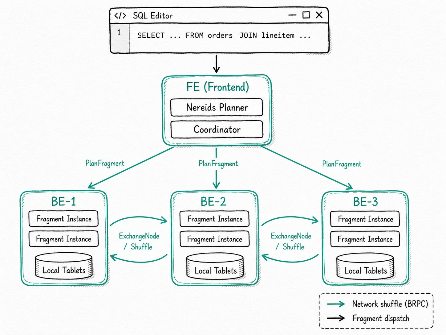
TL;DR Apache Doris MPP turns one SQL query into a DAG of PlanFragments that run in parallel on every BE in the cluster. The FE-side Coordinator plans the DAG with the Nereids optimizer, ships each fragment to its BEs over BRPC, and stitches fragments together with ExchangeNode + DataStreamSink shuffles. Shared-nothing storage and a per-query memory budget (exec_mem_limit, default 2 GB) let the cluster grow horizontally: every BE you add brings more CPU, memory, and local tablets to the same query pool.

Why use MPP in Apache Doris?

Apache Doris MPP exists so a single analytical query can use every CPU in the cluster instead of one machine's. A 10-billion-row aggregation, a five-way join across fact tables, a wide GROUP BY on a year of logs: none of these finish in human time on one node. The MPP layer is what turns "buy a bigger box" into "add more BEs."

The pain it solves is concrete:

• Single-node planners run out of headroom. A query that touches a terabyte of columnar data needs the scan, filter, join, and aggregate work spread across machines instead of stacked on one.
• Manual sharding is a tax on the data team. Hand-written union queries over per-shard tables work, until the join keys move or a shard rebalances.
• Storage-bound bottlenecks waste compute. Pulling shards into one box to compute means the network does the work the cluster could have done in place.

Apache Doris MPP gives the planner permission to split the query, send compute to the data, and shuffle only the rows that actually need to cross the wire.

What is the Apache Doris MPP architecture?

Apache Doris MPP is a shared-nothing distributed execution model where the Frontend (FE) plans the query as a DAG of PlanFragments and the Backends (BEs) run those fragments in parallel against their local tablets. The Nereids optimizer compiles the SQL into a logical plan, splits it on shuffle boundaries, and the FE Coordinator schedules each PlanFragment to a set of BEs. Each BE materializes the fragment into one or more fragment instances, which the BE-internal pipeline scheduler then runs on its threads. Data crosses fragment boundaries through ExchangeNodes (the consumer side) and DataStreamSinks (the producer side), serialized as Blocks and shipped over BRPC.

Key terms

• PlanFragment: the smallest unit of distributed work the FE ships to a BE. One query is one DAG of fragments.
• Fragment instance: a runtime copy of a PlanFragment running on one BE. Multiple instances of the same fragment on different BEs give you horizontal parallelism.
• Coordinator: the FE-side object that builds the fragment DAG, assigns BEs, ships fragments, collects results, and handles failures. Implemented in fe/fe-core/src/main/java/org/apache/doris/qe/Coordinator.java.
• ExchangeNode / DataStreamSink: the receiver / sender pair that moves data between fragments over the network. The planner inserts them on every shuffle boundary.
• Distribution mode: how rows are routed across the network on a shuffle: UNPARTITIONED, RANDOM, HASH_PARTITIONED, or BUCKET_SHFFULE_HASH_PARTITIONED.
• Nereids planner: the Cascades-style cost-based optimizer that picks the join order, the shuffle method, and the parallelism. The legacy planner has been deleted; the enable_nereids_planner switch is marked REMOVED.

How does the Apache Doris MPP architecture work?

Apache Doris MPP works in five stages: the FE plans, splits, and ships fragments; each BE turns its fragment into pipeline tasks; tablets are scanned locally; data is shuffled through ExchangeNodes only where the plan requires it; and a single root fragment returns the result to the client.

1. Plan and split. The Nereids optimizer rewrites the SQL into a physical plan and the FE walks the tree to cut it into PlanFragments at every point where data has to redistribute (an aggregation that needs all keys on one machine, a hash join that needs both sides hash-partitioned the same way, the final result sink).
2. Pick a shuffle method. For each fragment boundary the planner picks one of the four distribution modes, and for hash joins picks one of four strategies: Broadcast Join (copy the right side to every left instance), Shuffle Join (hash-partition both sides on the join key), Bucket Shuffle Join (reuse the left table's bucket layout to ship only the right side), or Colocate Join (skip the shuffle entirely because both tables already live on the same BEs). Cost determines which one runs.
3. Ship and instantiate. The Coordinator sends each fragment to its assigned BEs over BRPC. Each BE creates fragment instances, one per parallelism slot, and hands them to the Pipeline Execution Engine for scheduling.
4. Scan local, shuffle when needed. Scan operators read tablets that live on the same BE, so the bulk data never crosses the network. Only the rows the next fragment needs, serialized as columnar Blocks, cross the wire through DataStreamSink → ExchangeNode.
5. Return. A root fragment with an UNPARTITIONED sink runs on one BE, collects the merged result, and sends it back to the FE, which streams it to the client over the MySQL protocol.

Quick start

There is nothing to enable: MPP is how every query runs. The most useful operator-facing tool is EXPLAIN, which shows the fragment DAG, distribution modes, and shuffle strategies the optimizer picked.

EXPLAIN
SELECT o.o_orderpriority, COUNT(*) AS orders, SUM(l.l_extendedprice) AS revenue
FROM   orders o
JOIN   lineitem l ON o.o_orderkey = l.l_orderkey
WHERE  o.o_orderdate >= '2026-01-01'
GROUP BY o.o_orderpriority
ORDER BY revenue DESC
LIMIT 10;

Expected result (abridged)

PLAN FRAGMENT 2  (BUCKET_SHFFULE_HASH_PARTITIONED on o_orderkey)
  HASH JOIN   join op: INNER JOIN  ... (Bucket Shuffle)
    SCAN orders  (partitions=12, tablets=120, ...)
    EXCHANGE  HASH_PARTITIONED  <-- from FRAGMENT 1
PLAN FRAGMENT 1  (RANDOM)
  SCAN lineitem  (partitions=48, tablets=480, ...)
PLAN FRAGMENT 0  (UNPARTITIONED)
  RESULT SINK
  AGGREGATE (merge finalize)
    EXCHANGE  HASH_PARTITIONED  <-- from FRAGMENT 2

Three fragments. Fragment 1 scans lineitem on every BE that holds a tablet, hashes rows on l_orderkey, and pushes them into Fragment 2 over an exchange. Fragment 2 joins them against orders using Bucket Shuffle (orders is bucketed on o_orderkey, so its tablets don't move), pre-aggregates on o_orderpriority, and pushes the partial groups into Fragment 0. Fragment 0 finalizes the aggregation, sorts, and writes the result.

When should you use the Apache Doris MPP architecture?

Apache Doris MPP is the default execution mode for every analytical query: there is no other path for general SELECTs. Tune around it, not against it.

Good fit

• Analytical scans across tens of millions to billions of rows. Wide GROUP BYs, large joins, time-window aggregations.
• Star-schema and snowflake joins. Picking Bucket Shuffle or Colocate Join over Broadcast is exactly what the Nereids optimizer is built for.
• Multi-tenant clusters where queries should land on every BE. Pair MPP with Workload Group for CPU and memory isolation per tenant.
• Long-running queries on skewed data. The MPP planner's shuffle decisions feed the BE's Local Shuffle, which smooths skew inside each BE.

Not a good fit

• Single-row primary-key lookups at thousands of QPS. The cost of planning, shipping fragments, and round-tripping over BRPC dwarfs the work; use High-Concurrency Point Query instead.
• Treating MPP as a row-by-row OLTP engine. There is no per-row transaction layer; updates go through Unique Key tables and bulk load paths.
• Confusing MPP with Pipeline or vectorized execution. The three are stacked, not interchangeable. Pipeline Execution Engine runs operators inside one BE; Vectorized Execution runs the inner loop over column batches; MPP coordinates them across BEs.
• Tiny tables on a tiny cluster. If the whole table fits in one fragment's memory and one BE's CPU finishes the work in under a second, a Broadcast Join on a single BE is what the planner will pick, and that is the right answer.

Further reading

• Product concepts: Fragment, Instance, Exchange: the canonical user-facing definitions the rest of the docs build on.
• System architecture: FE/BE roles, BDBJE for FE consensus, and where the Coordinator sits in the topology.
• Join optimization and shuffle strategies: the cost trade-offs between Broadcast, Shuffle, Bucket Shuffle, and Colocate Join, with examples.
• Pipeline Execution Engine: the BE-internal scheduler MPP hands fragments to. Read this for the per-BE story.
• Parallelism tuning: when and how to override parallel_pipeline_task_num per workload.
• Evolution of the Apache Doris execution engine: the design history from volcano to Pipeline to PipelineX, with the MPP planner shifts along the way.