Runtime Filter Working Principles and Tuning

A Runtime Filter is a filter condition that Doris dynamically generates from runtime data during query execution, used to reduce the amount of scanned data and network transmission. Doris supports two types of Runtime Filter: Join Runtime Filter (JRF) and TopN Runtime Filter.

Pre-Reading Checklist

• Whether you understand the Doris Join execution flow and Scan node.
• Whether you can distinguish the execution modes of Hash Join and Shuffle Join.
• Whether you are familiar with how to inspect EXPLAIN, EXPLAIN SHAPE PLAN, and Profile.
• Whether you know whether the target scenario falls under Join filtering or TopN early pruning.

Join Runtime Filter

Join Runtime Filter (hereafter JRF) is a runtime optimization technique: at the Join node, Doris dynamically generates a filter from the right-side table data and pushes it down to the left-side table Scan, in order to reduce the Probe size, IO, and network transmission.

Working Principles

The following uses a TPC-H-like Schema Join to illustrate how JRF works.

Assume the database has two tables:

• Orders table (orders): 100 million rows, containing the order number o_orderkey, the customer ID o_custkey, and so on.
• Customer table (customer): 100,000 rows, containing the customer ID c_custkey, the customer nationality c_nation, and so on; there are 25 countries in total, with about 4,000 customers per country.

Count the number of orders from customers in China:

select count(*)
from orders join customer on o_custkey = c_custkey
where c_nation = "china"

The execution plan is essentially a Join:

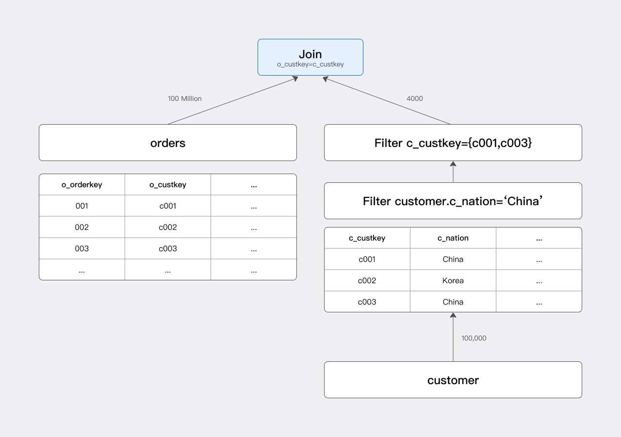
Without JRF, the Scan node scans all 100 million rows of the orders table, and the Join node performs a Hash Probe on them to produce the result.

1. Optimization Idea

The filter condition c_nation = "china" filters out all non-Chinese customers, so the customers participating in the Join are only a subset of the customer table (about 1/25). The Join condition is o_custkey = c_custkey, so we only need to care about the set of c_custkey values that pass the filter, denoted as set A.

Set A specifically refers to the set of c_custkey values participating in the Join.

If set A is pushed down as an IN condition to the orders table, the Scan node can pre-filter orders, which is equivalent to adding c_custkey in (c001, c003):

select count(*)
from orders join customer on o_custkey = c_custkey
where c_nation = "china" and o_custkey in (c001, c003)

The optimized execution plan:

The number of orders rows participating in the Join drops from 100 million to 400,000, which greatly improves query speed.

2. Implementation Method

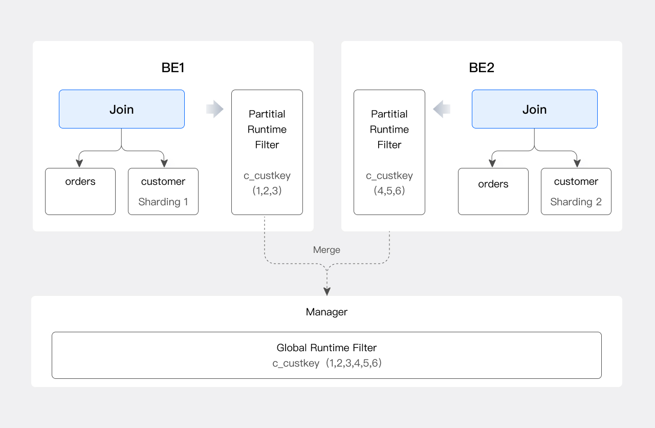
The optimizer cannot know the contents of set A during static analysis, so Doris generates set A at runtime after collecting the right-side data at the Join node, and pushes it down to the Scan node of the orders table. This JRF is usually denoted as: RF(c_custkey -> [o_custkey]).

Because Doris is a distributed database, the JRF also requires a merge step:

Step	Role	Action
1	Each Join Instance	Generates a Partial JRF based on the local shard c_custkey
2	Runtime Filter Manager (selected node)	Collects all Partial JRFs
3	Manager	Merges them into a Global JRF
4	Manager	Distributes the Global JRF to the Scan Instances of orders

The flow of generating a Global JRF:

Filter Types

JRF has multiple implementations, with different costs in generation, merging, transmission, and application.

Type	Applicable Scenarios	Filter Precision	Cost
In Filter	Equi-Join with few elements in set A	Exact	High deduplication, transmission, and Probe cost when there are many elements
Bloom Filter	Equi-Join with many elements in set A	Approximate (hash collisions exist)	Medium, affected by the number of buckets
Min-Max Filter	Sorted data, or non-equi-Join	Approximate	Lowest

1. In Filter

The simplest JRF implementation. Taking the previous example, the execution engine generates the predicate o_custkey in (...list of elements in A...) on the left table for filtering. It is efficient when set A is small.

When set A is large, the In Filter has performance issues:

1. High generation cost: When merging, the c_custkey values collected from each shard must be deduplicated (if c_custkey is not a primary key, there will be many duplicate values), which is time-consuming.
2. High transmission cost: Transmitting a large number of elements between the Join node and the Scan node is expensive.
3. High execution cost: Executing the IN predicate at the Scan node is itself time-consuming.

To address this, Doris introduces the Bloom Filter.

2. Bloom Filter

A Bloom Filter can be understood as a group of overlaid hash tables. It filters using the following property:

• Generate a hash table T from set A; if an element is not in T, it is definitely not in A; the converse does not hold.
• Therefore, an o_orderkey filtered out by the Bloom Filter definitely has no equal c_custkey on the right side of the Join; however, due to hash collisions, some non-matching o_custkey values may also pass the filter.
• The number of hash buckets determines the filter accuracy: more buckets means higher accuracy, but also higher generation, transmission, and computation cost.

The Bloom Filter size needs to be balanced between filtering effectiveness and cost. The maximum and minimum values can be constrained with the following parameters:

Parameter	Description
RUNTIME_BLOOM_FILTER_MIN_SIZE	Minimum number of bytes for the Bloom Filter
RUNTIME_BLOOM_FILTER_MAX_SIZE	Maximum number of bytes for the Bloom Filter

3. Min/Max Filter

The Min-Max Filter is also used for approximate filtering. It works well when the data column is sorted, and the cost of generation, merging, and application is far lower than that of the In Filter and Bloom Filter.

For non-equi-Joins, neither the In Filter nor the Bloom Filter works, but the Min-Max Filter is still effective:

select count(*)
from orders join customer on o_custkey > c_custkey
where c_name = "China"

It can pick out the maximum c_custkey after filtering, denoted as n, and pass it to the Scan node of orders; the Scan node only outputs rows where o_custkey > n.

Inspecting the Join Runtime Filter

You can inspect a JRF in the following three ways:

Method	Command	Description
Text execution plan	EXPLAIN	View the generation on the Join side and the application on the Scan side
Shape execution plan	EXPLAIN SHAPE PLAN	View the RF planned by the Nereids Planner
Actual execution Profile	Run the query after SET enable_profile=true	View the actual filtered row count and status

The following example is based on a TPC-H Schema:

select count(*) from orders join customer on o_custkey=c_custkey;

1. EXPLAIN

JRF information is distributed across the Join node and the Scan node:

4: VHASH JOIN(258)
| join op: INNER JOIN(PARTITIONED)[]
|  equal join conjunct: (o_custkey[#10] = c_custkey[#0])
|  runtime filters: RF000[bloom] <- c_custkey[#0] (150000000/134217728/16777216)
|  cardinality=1,500,000,000
|  vec output tuple id: 3
|  output tuple id: 3
|  vIntermediate tuple ids: 2
|  hash output slot ids: 10
|  final projections: o_custkey[#17]
|  final project output tuple id: 3
|  distribute expr lists: o_custkey[#10]
|  distribute expr lists: c_custkey[#0]
|
|---1: VEXCHANGE
|      offset: 0
|      distribute expr lists: c_custkey[#0]
3: VEXCHANGE
|  offset: 0
|  distribute expr lists:

PLAN FRAGMENT 2
| PARTITION: HASH_PARTITIONED: o_orderkey[#8]
| HAS_COLO_PLAN_NODE: false
| STREAM DATA SINK
|   EXCHANGE ID: 03
|   HASH_PARTITIONED: o_custkey[#10]

2: VOlapScanNode(242)
|  TABLE: regression_test_nereids_tpch_shape_sf1000_p0.orders(orders)
|  PREAGGREGATION: ON
|  runtime filters: RF000[bloom] -> o_custkey[#10]
|  partitions=1/1 (orders)
|  tablets=96/96, tabletList=54990,54992,54994 ...
|  cardinality=0, avgRowSize=0.0, numNodes=1
|  pushAggOp=NONE

Key field descriptions:

• Join side: runtime filters: RF000[bloom] <- c_custkey[#0] (150000000/134217728/16777216) This means a Bloom Filter numbered 000 is generated, taking the c_custkey field as input. The three numbers in parentheses relate to the Bloom Filter Size calculation and can be ignored for now.
• Scan side: runtime filters: RF000[bloom] -> o_custkey[#10] This means RF000 is applied to the Scan node of the orders table, filtering on the o_custkey field.

2. EXPLAIN SHAPE PLAN

mysql> explain shape plan select count(*) from orders join customer on o_custkey=c_custkey where c_nationkey=5;
+--------------------------------------------------------------------------------------------------------------------------+
Explain String(Nereids Planner)                                                                                            ｜
+--------------------------------------------------------------------------------------------------------------------------+
PhysicalResultSink                                                                                                         ｜
--hashAgg[GLOBAL]                                                                                                          ｜
----PhysicalDistribute[DistributionSpecGather]                                                                             ｜
------hashAgg[LOCAL]                                                                                                       ｜
--------PhysicalProject                                                                                                    ｜
----------hashJoin[INNER_JOIN shuffle]                                                                                     ｜
------------hashCondition=((orders.o_custkey=customer.c_custkey)) otherCondition=() buildRFs:RF0 c_custkey->[o_custkey]    ｜
--------------PhysicalProject                                                                                              ｜
----------------Physical0lapScan[orders] apply RFs: RF0                                                                    ｜
--------------PhysicalProject                                                                                              ｜
----------------filter((customer.c_nationkey=5))                                                                           ｜
------------------Physical0lapScan[customer]                                                                               ｜
+--------------------------------------------------------------------------------------------------------------------------+
11 rows in set (0.02 sec)

Key fields:

• Join side: buildRFs: RF0 c_custkey -> [o_custkey] means a JRF, numbered 0, is generated taking c_custkey as input and applied to o_custkey.
• Scan side: PhysicalOlapScan[orders] apply RFs: RF0 means the orders table is filtered by RF0.

3. Profile

During execution, the BE outputs JRF usage to the Profile (requires set enable_profile=true).

Join side Profile:

HASH_JOIN_SINK_OPERATOR  (id=3  ,  nereids_id=367):(ExecTime:  703.905us)
    -  JoinType:  INNER_JOIN
    ...
    -  BuildRows:  617
    ...
    -  RuntimeFilterComputeTime:  70.741us
    -  RuntimeFilterInitTime:  10.882us

In this example, generating the JRF takes 70.741us with 617 input rows; the JRF size and type are shown on the Scan side.

Scan side Profile:

OLAP_SCAN_OPERATOR  (id=2.  nereids_id=351.  table  name  =  orders(orders)):(ExecTime:  13.32ms)
              -  RuntimeFilters:  :  RuntimeFilter:  (id  =  0,  type  =  bloomfilter,  need_local_merge:  false,  is_broadcast:  true,  build_bf_cardinality:  false,
              ...
              -  RuntimeFilterInfo:
                  -  filter  id  =  0  filtered:  714.761K  (714761)
                  -  filter  id  =  0  input:  747.862K  (747862)
              ...
              -  WaitForRuntimeFilter:  6.317ms
            RuntimeFilter:  (id  =  0,  type  =  bloomfilter):
                  -  Info:  [IsPushDown  =  true,  RuntimeFilterState  =  READY,  HasRemoteTarget  =  false,  HasLocalTarget  =  true,  Ignored  =  false]
                  -  RealRuntimeFilterType:  bloomfilter
                  -  BloomFilterSize:  1024

Pay attention to the following information:

Focus	Field	Meaning
Filter effect	filter id = 0 filtered / input	A larger Filtered value indicates a better filtering effect
Whether pushed down to the storage layer	IsPushDown = true	After pushdown, lazy materialization can be triggered and IO reduced
Whether it takes effect	RuntimeFilterState = READY	A non-READY state means the Scan did not wait for the JRF
Filter size	BloomFilterSize: 1024	Number of bytes of the Bloom Filter

Tuning

In the vast majority of cases, JRF is adaptive and does not require manual tuning. If adjustment is truly required, you can use the following Session variables:

Variable	Default	Function
runtime_filter_mode	GLOBAL	Whether to enable JRF (GLOBAL enables / OFF disables)
runtime_filter_type	Default 12 in version 2.1	Controls the sum of JRF type enumeration values
runtime_filter_wait_time_ms	1000	The maximum number of milliseconds the Scan waits for the JRF
enable_runtime_filter_prune	true	Whether to prune JRFs that are not selective

1. Toggle JRF

• Enable: set runtime_filter_mode = GLOBAL
• Disable: set runtime_filter_mode = OFF

2. Set JRF Types

runtime_filter_type controls the JRF type enumeration values, which can be combined (summed) to generate multiple types simultaneously:

Type	Enumeration Value
IN	1
BLOOM	2
MIN_MAX	4
IN_OR_BLOOM	8

IN_OR_BLOOM lets the BE adaptively choose IN or BLOOM based on the actual number of rows. For example:

• set runtime_filter_type = 6: generates BLOOM and MIN_MAX simultaneously.
• The default value 12 (4 + 8) in version 2.1: generates MIN_MAX and IN_OR_BLOOM simultaneously.

3. Set the Wait Time

JRF uses a Try-best mechanism: the Scan waits for the JRF before starting; Doris automatically estimates the wait time. In some cases, insufficient waiting causes the JRF to not take effect, and the number of rows output by the Scan is higher than expected.

How to determine this: in the Profile, the Scan node shows RuntimeFilterState = false.

Operation:

• Purpose: extend the time the Scan waits for the JRF.
• Command: set runtime_filter_wait_time_ms = <milliseconds>
• Description: defaults to 1000 milliseconds.

4. Prune JRF

In some scenarios, the JRF is not selective. For example, if orders and customer have a primary-foreign key relationship and there is no filter condition on customer, the input to the JRF is all custkey values, which cannot filter orders. The optimizer determines effectiveness based on column statistics and prunes accordingly.

• Purpose: enable or disable JRF pruning.
• Command: set enable_runtime_filter_prune = true|false
• Description: defaults to true.

TopN Runtime Filter

The TopN Runtime Filter dynamically generates a filter based on the current heap-top value when the topN operator executes, pruning Scan data in advance.

Working Principles

Doris processes data in a chunked streaming manner. When the SQL contains topN, Doris does not compute all results, but instead generates a dynamic Filter to filter data in advance.

Example:

select o_orderkey from orders order by o_orderdate limit 5;

The execution plan is as follows:

mysql> explain select o_orderkey from orders order by o_orderdate limit 5;
+-----------------------------------------------------+
| Explain String(Nereids Planner)                     |
+-----------------------------------------------------+
| PLAN FRAGMENT 0                                     |
|   OUTPUT EXPRS:                                     |
|     o_orderkey[#11]                                 |
|   PARTITION: UNPARTITIONED                          |
|                                                     |
|   HAS_COLO_PLAN_NODE: false                         |
|                                                     |
|   VRESULT SINK                                      |
|      MYSQL_PROTOCAL                                 |
|                                                     |
|   2:VMERGING-EXCHANGE                               |
|      offset: 0                                      |
|      limit: 5                                       |
|      final projections: o_orderkey[#9]              |
|      final project output tuple id: 2               |
|      distribute expr lists:                         |
|                                                     |
| PLAN FRAGMENT 1                                     |
|                                                     |
|   PARTITION: HASH_PARTITIONED: O_ORDERKEY[#0]       |
|                                                     |
|   HAS_COLO_PLAN_NODE: false                         |
|                                                     |
|   STREAM DATA SINK                                  |
|     EXCHANGE ID: 02                                 |
|     UNPARTITIONED                                   |
|                                                     |
|   1:VTOP-N(119)                                     |
|   |  order by: o_orderdate[#10] ASC                 |
|   |  TOPN OPT                                       |
|   |  offset: 0                                      |
|   |  limit: 5                                       |
|   |  distribute expr lists: O_ORDERKEY[#0]          |
|   |                                                 |
|   0:VOlapScanNode(113)                              |
|      TABLE: tpch.orders(orders), PREAGGREGATION: ON |
|      TOPN OPT:1                                     |
|      partitions=1/1 (orders)                        |
|      tablets=3/3, tabletList=135112,135114,135116   |
|      cardinality=150000, avgRowSize=0.0, numNodes=1 |
|      pushAggOp=NONE                                 |
+-----------------------------------------------------+
41 rows in set (0.06 sec)

Execution flow:

1. Without a TopN Filter, the Scan reads data blocks one by one and feeds them to the TopN, which maintains the current Top 5 via heap sort.
2. A data Block contains about 1024 rows; after processing the first Block, the 5th-place value of that Block is known.
3. Suppose this value is 1995-01-01. When the Scan outputs the second Block, rows with o_orderdate > 1995-01-01 no longer need to be sent to the TopN.
4. The threshold updates dynamically: if subsequent Blocks contain a smaller o_orderdate, the TopN updates the threshold.

Inspecting the TopN Runtime Filter

Use EXPLAIN to inspect the TopN Runtime Filter planned by the optimizer:

1:VTOP-N(119)
| order by: o_orderdate[#10] ASC
| TOPN OPT
| offset: 0
| limit: 5
| distribute expr lists: O_ORDERKEY[#0]
|

0:VLapScanNode[113]
    TABLE: regression_test_nereids_tpch_p0.(orders), PREAGGREGATION: ON
    TOPN OPT: 1
    partitions=1/1 (orders)
    tablets=3/3, tabletList=135112,135114,135116
    cardinality=150000, avgRowSize=0.0, numNodes=1
    pushAggOp: NONE

Key fields:

• TopN node: shows TOPN OPT, indicating that this TopN node produces a TopN Runtime Filter.
• Scan node: indicates which TopN node produced the TopN Runtime Filter being used. For example, TOPN OPT: 1 indicates that the Scan of orders uses the Runtime Filter generated by the TopN node numbered 1.

As a distributed database, Doris also takes the physical locations of the TopN and the Scan into account. Cross-BE communication is expensive, so the BE adaptively decides whether to enable the filter and what its effective scope is. The current implementation is a BE-level TopN Runtime Filter (the TopN and Scan are within the same BE), relying only on inter-thread communication, which has low cost.

Tuning

The smaller the limit, the stronger the filtering of the TopN Runtime Filter. By default, the system enables it only when limit is less than half of the table data.

Variable	Function
topn_filter_ratio	Controls whether a TopN Runtime Filter is generated

For example, after setting set topn_filter_ratio=0, the following query does not generate a TopN Runtime Filter:

select o_orderkey from orders order by o_orderdate limit 20;

Runtime Filter Type Comparison

Dimension	Join Runtime Filter	TopN Runtime Filter
Trigger scenario	Join queries	ORDER BY ... LIMIT queries
Generation location	Join node	TopN node
Pushdown target	Left-table Scan	Scan within the same BE
Cross-BE	Supported (Global JRF merge)	Not supported (within a BE only)
Adaptive	Yes	Yes

FAQ / Troubleshooting

Q1: The JRF does not take effect, and the number of rows output by the Scan is far higher than expected. What should I do? Check RuntimeFilterState in the Profile: if it is not READY, the Scan timed out waiting. You can increase runtime_filter_wait_time_ms.

Q2: The JRF is generated but the Filtered row count is small. Why? The JRF input may not be selective (for example, a primary-foreign key Join with no filter condition on the right table). You can keep enable_runtime_filter_prune = true to let the optimizer prune automatically, or check whether a filter condition is missing on the right table.

Q3: How do I generate multiple JRF types at the same time? Set runtime_filter_type to the sum of the corresponding enumeration values. For example, set runtime_filter_type = 6 generates BLOOM and MIN_MAX simultaneously.

Q4: Can a non-equi-Join use JRF? You can use the Min-Max Filter; the In Filter and Bloom Filter only support equi-Joins.

Q5: The TopN Runtime Filter is not generated. Why? Check topn_filter_ratio: if it is 0, no filter is generated. By default, the system only generates the filter when limit is less than half of the table data; relaxing the limit or increasing topn_filter_ratio can trigger it.

Q6: How do I control the Bloom Filter size? Use RUNTIME_BLOOM_FILTER_MIN_SIZE and RUNTIME_BLOOM_FILTER_MAX_SIZE to limit the minimum and maximum number of bytes; this requires balancing filter precision against cost.