Analytic Functions (Window Functions)

Analytic functions, also known as window functions, are SQL functions that perform complex calculations across rows of a result set. The defining characteristic of a window function is that it does not reduce the number of rows returned by the query. Instead, it adds a new computed value to each row.

Window functions are useful in many data analysis scenarios, such as rolling totals, ranking, moving averages, and year-over-year or period-over-period comparisons. For detailed syntax, see Window Functions Overview.

Applicable Scenarios

Window functions are mainly used in the following data analysis scenarios:

Scenario	Typical Question	Recommended Functions
Ranking and grouping	"Rank the stores in each region by sales."	RANK / DENSE_RANK / ROW_NUMBER / NTILE
Cumulative statistics	"Compute the monthly cumulative sales for each product category."	SUM() OVER (... ROWS UNBOUNDED PRECEDING)
Moving average	"Compute a three-day-before-and-after moving average of store sales."	AVG() OVER (... ROWS BETWEEN n PRECEDING AND n FOLLOWING)
Reporting analysis	"Find the product category with the highest sales each year."	MAX() / SUM() OVER (PARTITION BY ...)
Row-to-row comparison	"Compute the year-over-year sales difference for each category."	LAG / LEAD

Quick Start: Moving Average Example

The following end-to-end example shows how to use a window function to compute the moving average of each store's sales over a window of three days before and three days after the current day.

1. Create the Table and Load Data

CREATE TABLE daily_sales (
    store_id INT,
    sales_date DATE,
    sales_amount DECIMAL(10, 2)
) PROPERTIES ("replication_num" = "1");

INSERT INTO daily_sales (store_id, sales_date, sales_amount) VALUES
(1, '2023-01-01', 100.00), (1, '2023-01-02', 150.00), (1, '2023-01-03', 200.00),
(1, '2023-01-04', 250.00), (1, '2023-01-05', 300.00), (1, '2023-01-06', 350.00),
(1, '2023-01-07', 400.00), (1, '2023-01-08', 450.00), (1, '2023-01-09', 500.00),
(2, '2023-01-01', 110.00), (2, '2023-01-02', 160.00), (2, '2023-01-03', 210.00),
(2, '2023-01-04', 260.00), (2, '2023-01-05', 310.00), (2, '2023-01-06', 360.00),
(2, '2023-01-07', 410.00), (2, '2023-01-08', 460.00), (2, '2023-01-09', 510.00);

2. Write the Query

SELECT
    store_id,
    sales_date,
    sales_amount,
    AVG(sales_amount) OVER (
        PARTITION BY store_id
        ORDER BY sales_date
        ROWS BETWEEN 3 PRECEDING AND 3 FOLLOWING
    ) AS moving_avg_sales
FROM daily_sales;

3. Query Result

+----------+------------+--------------+------------------+
| store_id | sales_date | sales_amount | moving_avg_sales |
+----------+------------+--------------+------------------+
|        1 | 2023-01-01 |       100.00 |         175.0000 |
|        1 | 2023-01-02 |       150.00 |         200.0000 |
|        1 | 2023-01-03 |       200.00 |         225.0000 |
|        1 | 2023-01-04 |       250.00 |         250.0000 |
|        1 | 2023-01-05 |       300.00 |         300.0000 |
|        1 | 2023-01-06 |       350.00 |         350.0000 |
|        1 | 2023-01-07 |       400.00 |         375.0000 |
|        1 | 2023-01-08 |       450.00 |         400.0000 |
|        1 | 2023-01-09 |       500.00 |         425.0000 |
|        2 | 2023-01-01 |       110.00 |         185.0000 |
|        2 | 2023-01-02 |       160.00 |         210.0000 |
|        2 | 2023-01-03 |       210.00 |         235.0000 |
|        2 | 2023-01-04 |       260.00 |         260.0000 |
|        2 | 2023-01-05 |       310.00 |         310.0000 |
|        2 | 2023-01-06 |       360.00 |         360.0000 |
|        2 | 2023-01-07 |       410.00 |         385.0000 |
|        2 | 2023-01-08 |       460.00 |         410.0000 |
|        2 | 2023-01-09 |       510.00 |         435.0000 |
+----------+------------+--------------+------------------+
18 rows in set (0.09 sec)

Basic Concepts

Before using window functions, you should understand a few core concepts: execution order, partitions, window frames, and the current row.

Processing Order

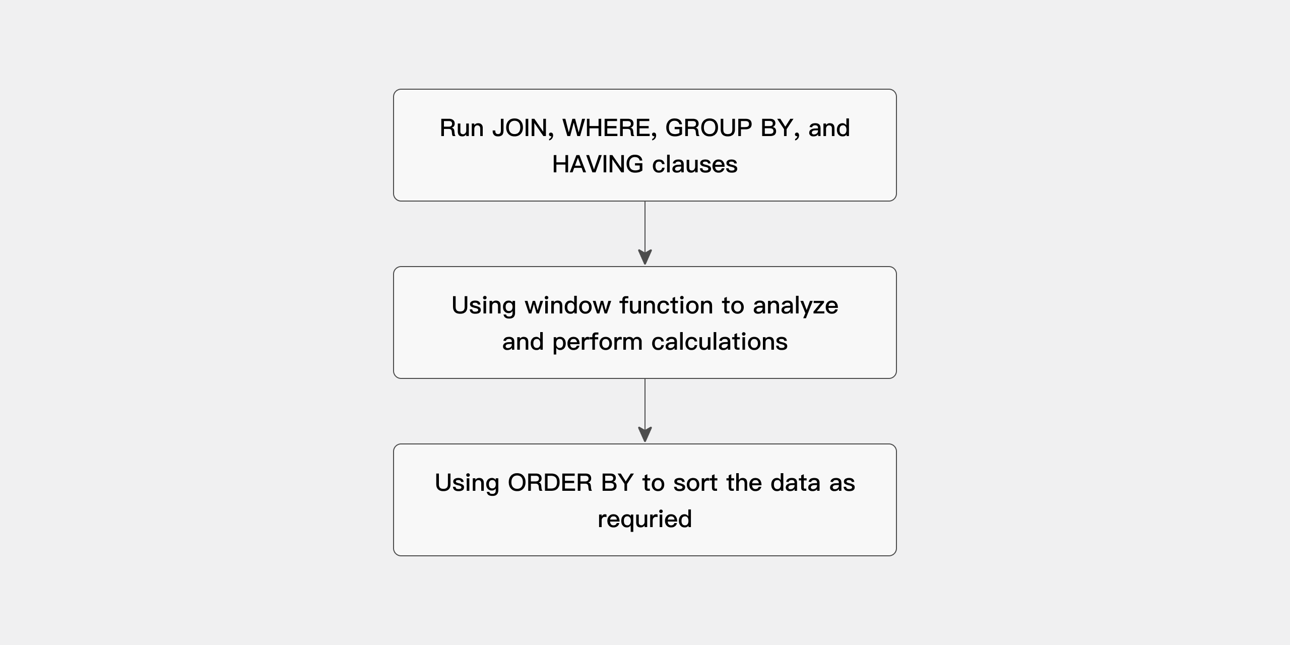
A query that uses analytic functions is processed in three phases:

1. All JOIN, WHERE, GROUP BY, and HAVING clauses are evaluated first.
2. The resulting set is passed to the analytic functions, which perform all window calculations.
3. If the query ends with an ORDER BY clause, that clause is processed last to determine the final output order.

The processing order is shown in the diagram below:

Result Set Partitioning

A partition is a logical group defined by the PARTITION BY clause. Rows within each partition are computed independently.

Note

The "partition" used in analytic functions has nothing to do with table partitioning. In this chapter, "partition" refers only to its meaning in the context of analytic functions.

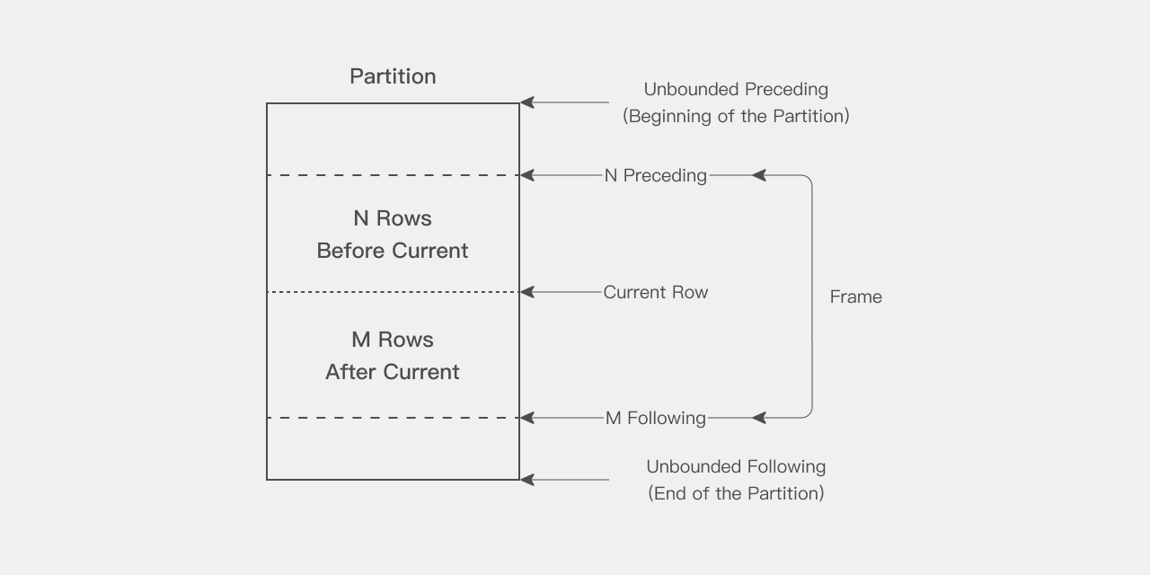
Window

For each row in a partition, you can define a sliding data window. The window determines the range of rows used in the calculation for the current row. A window has a start row and an end row, and depending on its definition, it may slide on one or both ends:

• ROWS BETWEEN UNBOUNDED PRECEDING AND CURRENT ROW: used for cumulative sums. The start of the window is fixed at the first row of the partition, and the end slides from the start row all the way to the last row of the partition.
• ROWS BETWEEN 3 PRECEDING AND 3 FOLLOWING: used for moving averages. Both the start and the end slide together with the current row.

The window can be as large as the entire partition or as small as a single row. Note that when the window is near the partition boundary, the number of rows that participate in the calculation may be reduced because of the boundary, and the function returns a result based only on the available rows.

When you use a window function, the current row is included in the calculation as well. Therefore, when you want to operate on n items, specify (n-1). For example, to compute a 5-day average, specify the window as ROWS BETWEEN 4 PRECEDING AND CURRENT ROW, which can also be shortened to ROWS 4 PRECEDING.

Current Row

Every calculation performed by an analytic function is based on the current row within a partition. The current row serves as the reference point for determining the start and end of the window.

For example, ROWS BETWEEN 6 PRECEDING AND 6 FOLLOWING defines a window for a centered moving average. The window contains the current row, the 6 rows before it, and the 6 rows after it, for a total of 13 rows.

Ranking Functions

Ranking functions sort or group rows within a partition. Note: the query result is deterministic only when the specified ordering column has unique values. If the ordering column contains duplicate values, the result may vary between executions. For more functions, see Window Functions Overview.

NTILE Function

NTILE divides the result set into a specified number of buckets (groups) and assigns a bucket number to each row. It is commonly used in data analysis and reporting for grouped ranking scenarios.

Syntax

NTILE(num_buckets) OVER ([PARTITION BY partition_expression] ORDER BY order_expression)

Parameter description:

Parameter	Description
num_buckets	The number of buckets into which the rows are divided.
PARTITION BY partition_expression	Optional. Defines how to partition the data.
ORDER BY order_expression	Required. Defines how to sort the data.

Example: Bucketing Students by Score

Suppose there is a table of student exam scores called class_student_scores, and you want to divide students into 4 groups by score, with each group containing roughly the same number of students.

First, create the table and insert data:

CREATE TABLE class_student_scores (
    class_id INT,
    student_id INT,
    student_name VARCHAR(50),
    score INT
) DISTRIBUTED BY HASH(student_id) PROPERTIES('replication_num'='1');

INSERT INTO class_student_scores VALUES
(1, 1, 'Alice', 85),
(1, 2, 'Bob', 92),
(1, 3, 'Charlie', 87),
(2, 4, 'David', 78),
(2, 5, 'Eve', 95),
(2, 6, 'Frank', 80),
(2, 7, 'Grace', 90),
(2, 8, 'Hannah', 84);

Then use the NTILE function to bucket students by score:

SELECT
    student_id,
    student_name,
    score,
    NTILE(4) OVER (ORDER BY score DESC) AS bucket
FROM class_student_scores;

Query result:

+------------+--------------+-------+--------+
| student_id | student_name | score | bucket |
+------------+--------------+-------+--------+
|          5 | Eve          |    95 |      1 |
|          2 | Bob          |    92 |      1 |
|          7 | Grace        |    90 |      2 |
|          3 | Charlie      |    87 |      2 |
|          1 | Alice        |    85 |      3 |
|          8 | Hannah       |    84 |      3 |
|          6 | Frank        |    80 |      4 |
|          4 | David        |    78 |      4 |
+------------+--------------+-------+--------+
8 rows in set (0.12 sec)

In this example, NTILE(4) divides the students into 4 buckets by score, with each bucket containing roughly the same number of students.

Notes

• If the rows cannot be distributed evenly across the buckets, some buckets may have one extra row.
• NTILE operates independently within each partition. When you use PARTITION BY, the data within each partition is bucketed separately.

Combining with PARTITION BY

If you want to "first group by class, then divide students within each class into 3 groups by score," you can combine NTILE with PARTITION BY:

SELECT
    class_id,
    student_id,
    student_name,
    score,
    NTILE(3) OVER (PARTITION BY class_id ORDER BY score DESC) AS bucket
FROM class_student_scores;

Query result:

+----------+------------+--------------+-------+--------+
| class_id | student_id | student_name | score | bucket |
+----------+------------+--------------+-------+--------+
|        1 |          2 | Bob          |    92 |      1 |
|        1 |          3 | Charlie      |    87 |      2 |
|        1 |          1 | Alice        |    85 |      3 |
|        2 |          5 | Eve          |    95 |      1 |
|        2 |          7 | Grace        |    90 |      1 |
|        2 |          8 | Hannah       |    84 |      2 |
|        2 |          6 | Frank        |    80 |      2 |
|        2 |          4 | David        |    78 |      3 |
+----------+------------+--------------+-------+--------+
8 rows in set (0.05 sec)

You can see that students are partitioned by class, and within each class they are divided into 3 buckets by score, with each bucket containing roughly the same number of students.

Aggregate Functions

Aggregate functions such as SUM, AVG, MAX, and MIN can be used as window functions when paired with the OVER clause. They compute aggregate values within a partition for each row without requiring a GROUP BY.

Use SUM to Compute a Cumulative Total

The following query computes the monthly sales for the Books and Electronics product categories in the year 2000, along with the cumulative total sales by month:

SELECT
    i_category,
    year(d_date),
    month(d_date),
    sum(ss_net_paid) AS total_sales,
    sum(sum(ss_net_paid)) OVER (
        PARTITION BY i_category
        ORDER BY year(d_date), month(d_date)
        ROWS UNBOUNDED PRECEDING
    ) AS cum_sales
FROM
    store_sales,
    date_dim d1,
    item
WHERE
    d1.d_date_sk = ss_sold_date_sk
    AND i_item_sk = ss_item_sk
    AND year(d_date) = 2000
    AND i_category IN ('Books', 'Electronics')
GROUP BY
    i_category,
    year(d_date),
    month(d_date);

Query result:

+-------------+--------------+---------------+-------------+-------------+
| i_category  | year(d_date) | month(d_date) | total_sales | cum_sales   |
+-------------+--------------+---------------+-------------+-------------+
| Books       |         2000 |             1 |  5348482.88 |  5348482.88 |
| Books       |         2000 |             2 |  4353162.03 |  9701644.91 |
| Books       |         2000 |             3 |  4466958.01 | 14168602.92 |
| Books       |         2000 |             4 |  4495802.19 | 18664405.11 |
| Books       |         2000 |             5 |  4589913.47 | 23254318.58 |
| Books       |         2000 |             6 |  4384384.00 | 27638702.58 |
| Books       |         2000 |             7 |  4488018.76 | 32126721.34 |
| Books       |         2000 |             8 |  9909227.94 | 42035949.28 |
| Books       |         2000 |             9 | 10366110.30 | 52402059.58 |
| Books       |         2000 |            10 | 10445320.76 | 62847380.34 |
| Books       |         2000 |            11 | 15246901.52 | 78094281.86 |
| Books       |         2000 |            12 | 15526630.11 | 93620911.97 |
| Electronics |         2000 |             1 |  5534568.17 |  5534568.17 |
| Electronics |         2000 |             2 |  4472655.10 | 10007223.27 |
| Electronics |         2000 |             3 |  4316942.60 | 14324165.87 |
| Electronics |         2000 |             4 |  4211523.06 | 18535688.93 |
| Electronics |         2000 |             5 |  4723661.00 | 23259349.93 |
| Electronics |         2000 |             6 |  4127773.06 | 27387122.99 |
| Electronics |         2000 |             7 |  4286523.05 | 31673646.04 |
| Electronics |         2000 |             8 | 10004890.96 | 41678537.00 |
| Electronics |         2000 |             9 | 10143665.77 | 51822202.77 |
| Electronics |         2000 |            10 | 10312020.35 | 62134223.12 |
| Electronics |         2000 |            11 | 14696000.54 | 76830223.66 |
| Electronics |         2000 |            12 | 15344441.52 | 92174665.18 |
+-------------+--------------+---------------+-------------+-------------+
24 rows in set (0.13 sec)

In this example, the SUM aggregate function defines a window for each row: the start is fixed at the first row of the partition (UNBOUNDED PRECEDING), and the end defaults to the current row. Note that SUM is nested here because the outer SUM aggregates the result of the inner SUM. Nested aggregation is very common in analytic aggregate functions.

Use AVG to Compute a Moving Average

The following query computes a "3-month moving average" (the current month and the previous two months) of the monthly sales for the Books category in the year 2000:

SELECT
    i_category,
    year(d_date),
    month(d_date),
    sum(ss_net_paid) AS total_sales,
    avg(sum(ss_net_paid)) OVER (
        ORDER BY year(d_date), month(d_date)
        ROWS 2 PRECEDING
    ) AS avg
FROM
    store_sales,
    date_dim d1,
    item
WHERE
    d1.d_date_sk = ss_sold_date_sk
    AND i_item_sk = ss_item_sk
    AND year(d_date) = 2000
    AND i_category = 'Books'
GROUP BY
    i_category,
    year(d_date),
    month(d_date);

Query result:

+------------+--------------+---------------+-------------+---------------+
| i_category | year(d_date) | month(d_date) | total_sales | avg           |
+------------+--------------+---------------+-------------+---------------+
| Books      |         2000 |             1 |  5348482.88 |  5348482.8800 |
| Books      |         2000 |             2 |  4353162.03 |  4850822.4550 |
| Books      |         2000 |             3 |  4466958.01 |  4722867.6400 |
| Books      |         2000 |             4 |  4495802.19 |  4438640.7433 |
| Books      |         2000 |             5 |  4589913.47 |  4517557.8900 |
| Books      |         2000 |             6 |  4384384.00 |  4490033.2200 |
| Books      |         2000 |             7 |  4488018.76 |  4487438.7433 |
| Books      |         2000 |             8 |  9909227.94 |  6260543.5666 |
| Books      |         2000 |             9 | 10366110.30 |  8254452.3333 |
| Books      |         2000 |            10 | 10445320.76 | 10240219.6666 |
| Books      |         2000 |            11 | 15246901.52 | 12019444.1933 |
| Books      |         2000 |            12 | 15526630.11 | 13739617.4633 |
+------------+--------------+---------------+-------------+---------------+
12 rows in set (0.13 sec)

Note

In the output, the avg column for the first two rows is not actually computed as a true 3-month average, because there are not enough preceding rows (the SQL specifies a window of 3 rows).

You can also compute a window aggregation that is "centered on the current row." The example below computes a centered moving average of the monthly sales for the Books category in the year 2000, that is, the average of the sales for "the previous month, the current month, and the next month":

SELECT
    i_category,
    year(d_date),
    month(d_date),
    sum(ss_net_paid) AS total_sales,
    avg(sum(ss_net_paid)) OVER (
        ORDER BY year(d_date), month(d_date)
        ROWS BETWEEN 1 PRECEDING AND 1 FOLLOWING
    ) AS avg_sales
FROM
    store_sales,
    date_dim d1,
    item
WHERE
    d1.d_date_sk = ss_sold_date_sk
    AND i_item_sk = ss_item_sk
    AND year(d_date) = 2000
    AND i_category = 'Books'
GROUP BY
    i_category,
    year(d_date),
    month(d_date);

Note

In the output, the centered moving average for the first and last rows is computed based on only two months of data, because there are not enough rows on one side of the boundary.

Reporting Functions

A reporting function has the property that "the window for every row spans the entire partition." Its main advantage is that the same data can be referenced multiple times in a single query, which avoids explicit JOINs and improves query performance.

For example, the requirement "find the product category with the highest sales each year" can be implemented with a reporting function and does not require a JOIN:

SELECT year, category, total_sum FROM (
    SELECT
        year(d_date) AS year,
        i_category AS category,
        sum(ss_net_paid) AS total_sum,
        max(sum(ss_net_paid)) OVER (PARTITION BY year(d_date)) AS max_sales
    FROM
        store_sales,
        date_dim d1,
        item
    WHERE
        d1.d_date_sk = ss_sold_date_sk
        AND i_item_sk = ss_item_sk
        AND year(d_date) IN (1998, 1999)
    GROUP BY
        year(d_date), i_category
) t
WHERE total_sum = max_sales;

The inner query reports the highest category sales for each year using MAX(SUM(ss_net_paid)), with the following result:

+------+-------------+-------------+-------------+
| year | category    | total_sum   | max_sales   |
+------+-------------+-------------+-------------+
| 1998 | Electronics | 91723676.27 | 91723676.27 |
| 1998 | Books       | 91307909.84 | 91723676.27 |
| 1999 | Electronics | 90310850.54 | 90310850.54 |
| 1999 | Books       | 88993351.11 | 90310850.54 |
+------+-------------+-------------+-------------+
4 rows in set (0.11 sec)

After the outer query filters with total_sum = max_sales, you get the top-selling category for each year:

+------+-------------+-------------+
| year | category    | total_sum   |
+------+-------------+-------------+
| 1998 | Electronics | 91723676.27 |
| 1999 | Electronics | 90310850.54 |
+------+-------------+-------------+
2 rows in set (0.12 sec)

Reporting aggregations can also be combined with nested queries to solve more complex problems. For example, "find the subcategories whose product sales account for more than 20% of their product category's total sales, and select the top 5 best-selling items from those subcategories":

SELECT i_category AS categ, i_class AS sub_categ, i_item_id
FROM (
    SELECT
        i_item_id, i_class, i_category,
        sum(ss_net_paid) AS sales,
        sum(sum(ss_net_paid)) OVER (PARTITION BY i_category) AS cat_sales,
        sum(sum(ss_net_paid)) OVER (PARTITION BY i_class) AS sub_cat_sales,
        rank() OVER (PARTITION BY i_class ORDER BY sum(ss_net_paid) DESC) AS rank_in_line
    FROM
        store_sales,
        item
    WHERE
        i_item_sk = ss_item_sk
    GROUP BY i_class, i_category, i_item_id
) t
WHERE sub_cat_sales > 0.2 * cat_sales AND rank_in_line <= 5;

LAG / LEAD Functions

The LAG and LEAD functions are designed for "row-to-row comparison" scenarios. Both functions can access multiple rows in a table without a self-join, which significantly improves query efficiency:

• LAG: accesses the row at a given offset before the current row.
• LEAD: accesses the row at a given offset after the current row.

Example 1: Use LAG to Compute Year-over-Year Sales Differences

The following query selects the total sales, the previous year's total sales, and the difference between the two for each product category in the years 1999, 2000, 2001, and 2002:

SELECT year, category, total_sales, before_year_sales, total_sales - before_year_sales FROM (
    SELECT
        sum(ss_net_paid) AS total_sales,
        year(d_date) AS year,
        i_category AS category,
        lag(sum(ss_net_paid), 1, 0) OVER (
            PARTITION BY i_category
            ORDER BY YEAR(d_date)
        ) AS before_year_sales
    FROM
        store_sales,
        date_dim d1,
        item
    WHERE
        d1.d_date_sk = ss_sold_date_sk
        AND i_item_sk = ss_item_sk
    GROUP BY
        YEAR(d_date), i_category
) t
WHERE year IN (1999, 2000, 2001, 2002);

Query result:

+------+-------------+-------------+-------------------+-----------------------------------+
| year | category    | total_sales | before_year_sales | (total_sales - before_year_sales) |
+------+-------------+-------------+-------------------+-----------------------------------+
| 1999 | Books       | 88993351.11 |       91307909.84 |                       -2314558.73 |
| 2000 | Books       | 93620911.97 |       88993351.11 |                        4627560.86 |
| 2001 | Books       | 90640097.99 |       93620911.97 |                       -2980813.98 |
| 2002 | Books       | 89585515.90 |       90640097.99 |                       -1054582.09 |
| 1999 | Electronics | 90310850.54 |       91723676.27 |                       -1412825.73 |
| 2000 | Electronics | 92174665.18 |       90310850.54 |                        1863814.64 |
| 2001 | Electronics | 92598527.85 |       92174665.18 |                         423862.67 |
| 2002 | Electronics | 94303831.84 |       92598527.85 |                        1705303.99 |
+------+-------------+-------------+-------------------+-----------------------------------+
8 rows in set (0.16 sec)

Example 2: Use a Window Function to Compute a 3-Day Stock Price Average

Suppose there is the following stock data, where the ticker symbol is JDR and closing_price is the daily closing price:

CREATE TABLE stock_ticker (
    stock_symbol STRING,
    closing_price DECIMAL(8, 2),
    closing_date DATETIME
);

INSERT INTO stock_ticker VALUES
    ("JDR", 12.86, "2014-10-02 00:00:00"),
    ("JDR", 12.89, "2014-10-03 00:00:00"),
    ("JDR", 12.94, "2014-10-04 00:00:00"),
    ("JDR", 12.55, "2014-10-05 00:00:00"),
    ("JDR", 14.03, "2014-10-06 00:00:00"),
    ("JDR", 14.75, "2014-10-07 00:00:00"),
    ("JDR", 13.98, "2014-10-08 00:00:00");

SELECT * FROM stock_ticker ORDER BY stock_symbol, closing_date;

| stock_symbol | closing_price | closing_date        |
|--------------|---------------|---------------------|
| JDR          | 12.86         | 2014-10-02 00:00:00 |
| JDR          | 12.89         | 2014-10-03 00:00:00 |
| JDR          | 12.94         | 2014-10-04 00:00:00 |
| JDR          | 12.55         | 2014-10-05 00:00:00 |
| JDR          | 14.03         | 2014-10-06 00:00:00 |
| JDR          | 14.75         | 2014-10-07 00:00:00 |
| JDR          | 13.98         | 2014-10-08 00:00:00 |

The query below uses a window function to produce a moving_average column, whose value is the average of the stock prices for the previous day, the current day, and the next day. The first day has no previous day and the last day has no next day, so those two rows are actually averaged over only two days. PARTITION BY does not have a real grouping effect here (because all the data belongs to JDR), but when there are multiple stocks, PARTITION BY ensures that the window calculation is performed only within the same stock:

SELECT
    stock_symbol,
    closing_date,
    closing_price,
    avg(closing_price) OVER (
        PARTITION BY stock_symbol
        ORDER BY closing_date
        ROWS BETWEEN 1 PRECEDING AND 1 FOLLOWING
    ) AS moving_average
FROM stock_ticker;

| stock_symbol | closing_date        | closing_price | moving_average |
|--------------|---------------------|---------------|----------------|
| JDR          | 2014-10-02 00:00:00 | 12.86         | 12.87          |
| JDR          | 2014-10-03 00:00:00 | 12.89         | 12.89          |
| JDR          | 2014-10-04 00:00:00 | 12.94         | 12.79          |
| JDR          | 2014-10-05 00:00:00 | 12.55         | 13.17          |
| JDR          | 2014-10-06 00:00:00 | 14.03         | 13.77          |
| JDR          | 2014-10-07 00:00:00 | 14.75         | 14.25          |
| JDR          | 2014-10-08 00:00:00 | 13.98         | 14.36          |

Appendix: Sample Data Preparation

The aggregate function, reporting function, and LAG/LEAD examples in this document are all based on TPC-DS-style tables (item, store_sales, date_dim, customer_address). To reproduce them, follow the steps below to prepare the data.

1. Create the Sample Tables

CREATE DATABASE IF NOT EXISTS doc_tpcds;
USE doc_tpcds;

CREATE TABLE IF NOT EXISTS item (
    i_item_sk bigint not null,
    i_item_id char(16) not null,
    i_rec_start_date date,
    i_rec_end_date date,
    i_item_desc varchar(200),
    i_current_price decimal(7,2),
    i_wholesale_cost decimal(7,2),
    i_brand_id integer,
    i_brand char(50),
    i_class_id integer,
    i_class char(50),
    i_category_id integer,
    i_category char(50),
    i_manufact_id integer,
    i_manufact char(50),
    i_size char(20),
    i_formulation char(20),
    i_color char(20),
    i_units char(10),
    i_container char(10),
    i_manager_id integer,
    i_product_name char(50)
)
DUPLICATE KEY(i_item_sk)
DISTRIBUTED BY HASH(i_item_sk) BUCKETS 12
PROPERTIES (
    "replication_num" = "1"
);

CREATE TABLE IF NOT EXISTS store_sales (
    ss_item_sk bigint not null,
    ss_ticket_number bigint not null,
    ss_sold_date_sk bigint,
    ss_sold_time_sk bigint,
    ss_customer_sk bigint,
    ss_cdemo_sk bigint,
    ss_hdemo_sk bigint,
    ss_addr_sk bigint,
    ss_store_sk bigint,
    ss_promo_sk bigint,
    ss_quantity integer,
    ss_wholesale_cost decimal(7,2),
    ss_list_price decimal(7,2),
    ss_sales_price decimal(7,2),
    ss_ext_discount_amt decimal(7,2),
    ss_ext_sales_price decimal(7,2),
    ss_ext_wholesale_cost decimal(7,2),
    ss_ext_list_price decimal(7,2),
    ss_ext_tax decimal(7,2),
    ss_coupon_amt decimal(7,2),
    ss_net_paid decimal(7,2),
    ss_net_paid_inc_tax decimal(7,2),
    ss_net_profit decimal(7,2)
)
DUPLICATE KEY(ss_item_sk, ss_ticket_number)
DISTRIBUTED BY HASH(ss_item_sk, ss_ticket_number) BUCKETS 32
PROPERTIES (
    "replication_num" = "1"
);

CREATE TABLE IF NOT EXISTS date_dim (
    d_date_sk bigint not null,
    d_date_id char(16) not null,
    d_date date,
    d_month_seq integer,
    d_week_seq integer,
    d_quarter_seq integer,
    d_year integer,
    d_dow integer,
    d_moy integer,
    d_dom integer,
    d_qoy integer,
    d_fy_year integer,
    d_fy_quarter_seq integer,
    d_fy_week_seq integer,
    d_day_name char(9),
    d_quarter_name char(6),
    d_holiday char(1),
    d_weekend char(1),
    d_following_holiday char(1),
    d_first_dom integer,
    d_last_dom integer,
    d_same_day_ly integer,
    d_same_day_lq integer,
    d_current_day char(1),
    d_current_week char(1),
    d_current_month char(1),
    d_current_quarter char(1),
    d_current_year char(1)
)
DUPLICATE KEY(d_date_sk)
DISTRIBUTED BY HASH(d_date_sk) BUCKETS 12
PROPERTIES (
    "replication_num" = "1"
);

CREATE TABLE IF NOT EXISTS customer_address (
    ca_address_sk bigint not null,
    ca_address_id char(16) not null,
    ca_street_number char(10),
    ca_street_name varchar(60),
    ca_street_type char(15),
    ca_suite_number char(10),
    ca_city varchar(60),
    ca_county varchar(30),
    ca_state char(2),
    ca_zip char(10),
    ca_country varchar(20),
    ca_gmt_offset decimal(5,2),
    ca_location_type char(20)
)
DUPLICATE KEY(ca_address_sk)
DISTRIBUTED BY HASH(ca_address_sk) BUCKETS 12
PROPERTIES (
    "replication_num" = "1"
);

2. Download and Load the Data via Stream Load

In a terminal, run the following commands to download the data locally and load it using Stream Load:

curl -L https://cdn.selectdb.com/static/doc_ddl_dir_d27a752a7b.tar -o - | tar -Jxf -

curl --location-trusted \
    -u "root:" \
    -H "column_separator:|" \
    -H "columns: i_item_sk, i_item_id, i_rec_start_date, i_rec_end_date, i_item_desc, i_current_price, i_wholesale_cost, i_brand_id, i_brand, i_class_id, i_class, i_category_id, i_category, i_manufact_id, i_manufact, i_size, i_formulation, i_color, i_units, i_container, i_manager_id, i_product_name" \
    -T "doc_ddl_dir/item_1_10.dat" \
    http://127.0.0.1:8030/api/doc_tpcds/item/_stream_load

curl --location-trusted \
    -u "root:" \
    -H "column_separator:|" \
    -H "columns: d_date_sk, d_date_id, d_date, d_month_seq, d_week_seq, d_quarter_seq, d_year, d_dow, d_moy, d_dom, d_qoy, d_fy_year, d_fy_quarter_seq, d_fy_week_seq, d_day_name, d_quarter_name, d_holiday, d_weekend, d_following_holiday, d_first_dom, d_last_dom, d_same_day_ly, d_same_day_lq, d_current_day, d_current_week, d_current_month, d_current_quarter, d_current_year" \
    -T "doc_ddl_dir/date_dim_1_10.dat" \
    http://127.0.0.1:8030/api/doc_tpcds/date_dim/_stream_load

curl --location-trusted \
    -u "root:" \
    -H "column_separator:|" \
    -H "columns: ss_sold_date_sk, ss_sold_time_sk, ss_item_sk, ss_customer_sk, ss_cdemo_sk, ss_hdemo_sk, ss_addr_sk, ss_store_sk, ss_promo_sk, ss_ticket_number, ss_quantity, ss_wholesale_cost, ss_list_price, ss_sales_price, ss_ext_discount_amt, ss_ext_sales_price, ss_ext_wholesale_cost, ss_ext_list_price, ss_ext_tax, ss_coupon_amt, ss_net_paid, ss_net_paid_inc_tax, ss_net_profit" \
    -T "doc_ddl_dir/store_sales.csv" \
    http://127.0.0.1:8030/api/doc_tpcds/store_sales/_stream_load

curl --location-trusted \
    -u "root:" \
    -H "column_separator:|" \
    -H "ca_address_sk, ca_address_id, ca_street_number, ca_street_name, ca_street_type, ca_suite_number, ca_city, ca_county, ca_state, ca_zip, ca_country, ca_gmt_offset, ca_location_type" \
    -T "doc_ddl_dir/customer_address_1_10.dat" \
    http://127.0.0.1:8030/api/doc_tpcds/customer_address/_stream_load

The data files item_1_10.dat, date_dim_1_10.dat, store_sales.csv, and customer_address_1_10.dat can also be downloaded from this archive.