Basic Concepts
This document introduces the partitioning (Partition) and bucketing (Bucket) mechanisms of Doris, helping you design table structures reasonably to improve query performance and data management efficiency. New users are recommended to read the sections in order: Sections 1-3 cover core concepts and the first CREATE TABLE example, Sections 4-6 cover advanced features and design recommendations, and Section 7 covers the methods for viewing and modifying partitions needed for daily operations.
1. Overview
Doris uses a two-tier data partitioning approach of Partition + Bucket to organize the data of a table in an orderly manner across the nodes of the cluster:
- Partition: horizontally divides the table into smaller subsets by column values (such as time or region), making it easier to perform query pruning and data lifecycle management.
- Bucket: further evenly distributes data within each partition into multiple data shards (Tablets), fully utilizing the parallelism of the cluster.
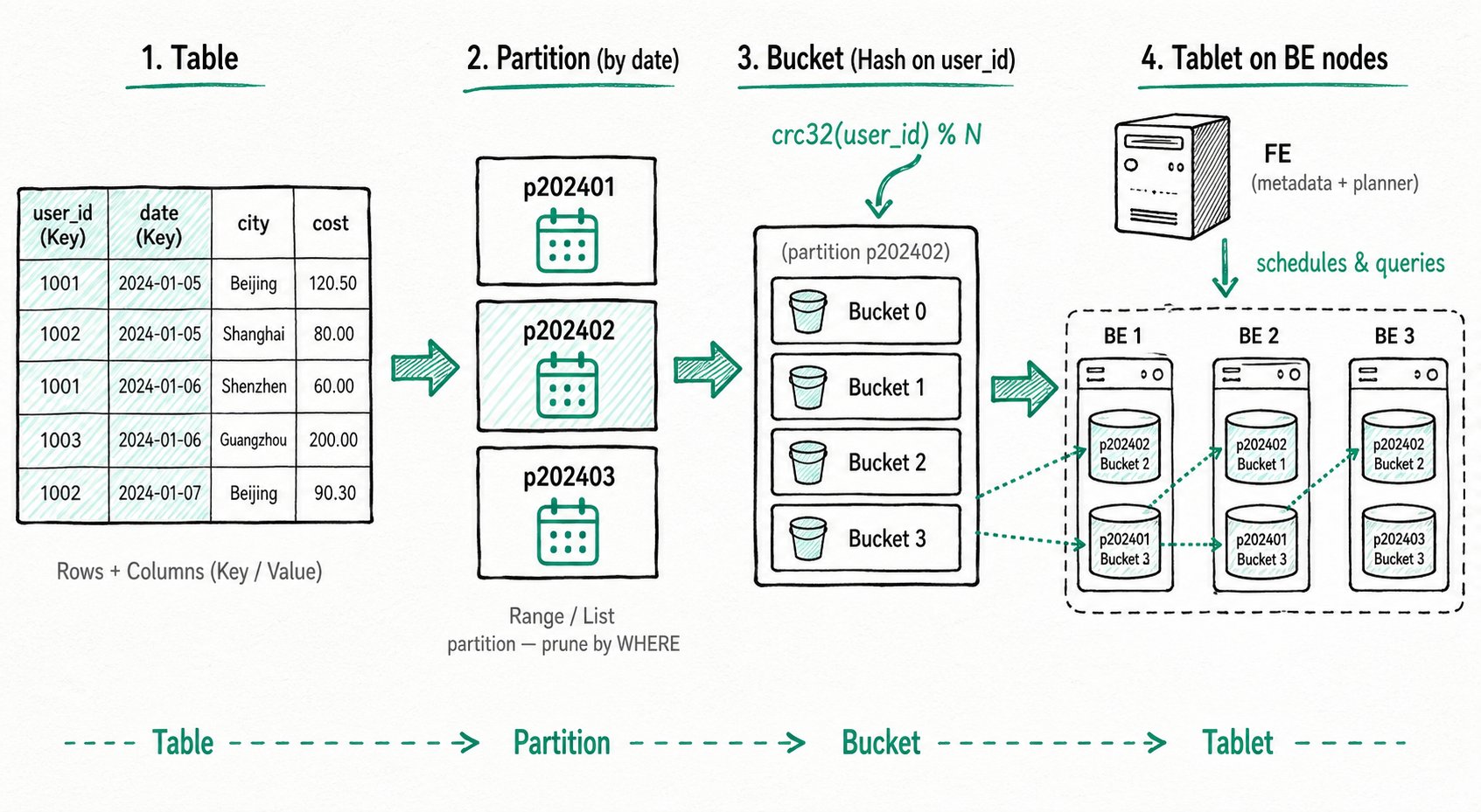
The data flow can be summarized as:
Table ──► Partition ──► Bucket ──► Tablet (data shard, stored on BE nodes)
A reasonable partitioning and bucketing design brings the following benefits at the same time: faster queries (partition pruning, parallel scanning), more flexible management (archiving/cleanup by time), and more even writes (avoiding hotspots).
2. Core Concepts
2.1 Table Structure: Rows and Columns
In Doris, data is logically described in the form of tables. A table consists of rows (Row) and columns (Column):
| Concept | Description |
|---|---|
| Row | A row of user data |
| Column | Describes different fields in a row of data |
Columns can be further divided into two categories:
| Column Type | Business Mapping | Description |
|---|---|---|
| Key column | Dimension column | Columns specified after the unique key, aggregate key, or duplicate key keyword in the CREATE TABLE statement |
| Value column | Metric column | Columns other than the Key columns; the aggregation method is specified at table creation time |
In the Aggregate model, rows with identical Key columns are aggregated into one row, and the aggregation method for Value columns is specified by the user at table creation time. For more information about the Aggregate model, see Doris Data Model.
2.2 Partition
A partition divides data into smaller, mutually disjoint subsets based on the values of specific columns in the table. Each row of data belongs to exactly one specific partition, and the partition is the smallest logical management unit.
Doris supports two partition types:
- Range partition: divides by numeric or time range, commonly used for time-series data.
- List partition: divides by sets of enumerated values, commonly used to split by discrete dimensions such as region or category.
If no partition is specified at table creation time, Doris generates a default partition that is transparent to the user, containing all the data in the table.
A reasonable partition design brings the following benefits:
- Improved query performance: through partition pruning, the system can filter out irrelevant partitions based on query conditions, reducing the amount of data scanned and significantly lowering the I/O burden, which is especially suitable for large-scale datasets.
- Management flexibility: data can be split along logical dimensions such as time or region, making archiving, cleanup, and backup easier. For example, partitioning by time enables efficient management of historical and incremental data, supporting time-based data maintenance strategies.
2.3 Bucket
Bucketing further divides the data within a partition into smaller, mutually disjoint data units according to certain rules. Each row of data belongs to exactly one specific bucket.
Unlike partitions that divide by ranges of column values, the goal of bucketing is to evenly distribute data across predefined buckets, thereby reducing data skew and improving query execution performance through better data locality.
Doris supports two bucketing methods:
- Hash bucketing: computes the
crc32hash of the bucketing column values and takes the modulo with the number of buckets to evenly distribute the data. - Random bucketing: randomly assigns data to buckets. When using Random bucketing, you can combine the
load_to_single_tabletparameter to optimize fast writes for small-scale data.
A reasonable bucketing design brings the following benefits:
- Even data distribution: reduces the risk of data concentration or skew, and avoids overloading some nodes or storage devices.
- Reduced hotspots: prevents some nodes or partitions from being overloaded, improving system stability and processing capability.
- Improved concurrent performance: when multiple query requests need to access different data within the same partition, bucketing allows the system to process multiple requests in parallel effectively, thereby improving throughput.
2.4 Tablet and Node Architecture
A bucket physically corresponds to a Tablet (data shard). The Tablet is the smallest unit of data management in Doris, and is also the basic physical unit for operations such as data movement and replication.
A Doris cluster consists of two types of nodes:
- FE node (Frontend): manages cluster metadata (such as table and tablet information), and is responsible for SQL parsing and execution planning.
- BE node (Backend): stores Tablet data and is responsible for executing computation tasks. The results from BEs are aggregated and returned to the user by the FE.
When data is written and queried, partitions and buckets work together as follows:
- Data writing: data rows are first assigned to the corresponding partition according to the partitioning strategy, and then mapped to a specific Tablet within the partition according to the bucketing strategy.
- Query execution: the FE optimizer prunes irrelevant partitions and buckets based on query conditions, minimizing the scan range. When JOIN or aggregation queries are involved, cross-node Shuffle may occur. A reasonable partitioning and bucketing design (combined with Colocate when necessary) can significantly reduce Shuffle costs.
3. The First CREATE TABLE Example
Creating a table in Doris is a synchronous command. The result is returned upon completion of the SQL statement, and successful return indicates the table is created. For the complete CREATE TABLE syntax, see CREATE TABLE, or use HELP CREATE TABLE for more help information.
The following is a minimal CREATE TABLE example using Range partitioning + Hash bucketing:
-- Range Partition
CREATE TABLE example_range_tbl
(
    `user_id` LARGEINT NOT NULL COMMENT "User ID",
    `date` DATE NOT NULL COMMENT "Data ingestion date",
    `timestamp` DATETIME NOT NULL COMMENT "Data ingestion timestamp",
    `city` VARCHAR(20) COMMENT "User's city",
    `age` SMALLINT COMMENT "User age",
    `sex` TINYINT COMMENT "User gender",
    `last_visit_date` DATETIME REPLACE DEFAULT "1970-01-01 00:00:00" COMMENT "User's last visit time",
    `cost` BIGINT SUM DEFAULT "0" COMMENT "Total user spending",
    `max_dwell_time` INT MAX DEFAULT "0" COMMENT "Maximum user dwell time",
    `min_dwell_time` INT MIN DEFAULT "99999" COMMENT "Minimum user dwell time"
)
PARTITION BY RANGE(`date`)
(
    PARTITION `p201701` VALUES LESS THAN ("2017-02-01"),
    PARTITION `p201702` VALUES LESS THAN ("2017-03-01"),
    PARTITION `p201703` VALUES LESS THAN ("2017-04-01"),
    PARTITION `p2018` VALUES [("2018-01-01"), ("2019-01-01"))
)
DISTRIBUTED BY HASH(`user_id`) BUCKETS 16
PROPERTIES
(
    "replication_num" = "1"
);
Understanding the write and query process with this example:
- During writes, each row of data first falls into the corresponding Range partition by
date(for example,2017-02-15falls intop201702), and is then mapped to one of the 16 Tablets under that partition by the hash value ofuser_id. - For a query with
WHERE date = '2017-02-15', the optimizer scans only thep201702partition. Ifuser_id = 123is also added, only one Tablet is hit.
4. Advanced: Partition Modes
Besides manually declaring partitions at table creation time, Doris also supports automatic partition creation based on time scheduling (Dynamic Partition) and on-demand partition creation based on incoming data (Auto Partition). The three modes are compared as follows:
| Partition Mode | When Partitions Are Created | Applicable Scenarios |
|---|---|---|
| Manual partition | Explicitly declared at table creation, or added via ALTER | Stable partition set, requiring fine-grained control |
| Dynamic partition | Automatically created/recycled by the system based on time scheduling rules | Time-series data, where you want to automatically maintain rolling partitions for the past N days/weeks/months |
| Auto partition | Created on demand when data is written | Partition values are unpredictable (such as multi-tenant or sparse time), where pre-creation should be avoided |
The following shows CREATE TABLE examples for common combinations:
- Auto Partition
- Dynamic Partition
- Auto Partition + Dynamic Partition
Auto Partition supports automatically creating corresponding partitions according to user-defined rules during data ingestion, making it more convenient to use. The basic example rewritten as Auto Range partition:
CREATE TABLE example_range_tbl
(
    `user_id` LARGEINT NOT NULL COMMENT "User ID",
    `date` DATE NOT NULL COMMENT "Data ingestion date",
    `timestamp` DATETIME NOT NULL COMMENT "Data ingestion timestamp",
    `city` VARCHAR(20) COMMENT "User's city",
    `age` SMALLINT COMMENT "User age",
    `sex` TINYINT COMMENT "User gender",
    `last_visit_date` DATETIME REPLACE DEFAULT "1970-01-01 00:00:00" COMMENT "User's last visit time",
    `cost` BIGINT SUM DEFAULT "0" COMMENT "Total user spending",
    `max_dwell_time` INT MAX DEFAULT "0" COMMENT "Maximum user dwell time",
    `min_dwell_time` INT MIN DEFAULT "99999" COMMENT "Minimum user dwell time"
)
AUTO PARTITION BY RANGE(date_trunc(`date`, 'month')) --- Use month as the partition granularity
()
DISTRIBUTED BY HASH(`user_id`) BUCKETS 16
PROPERTIES
(
    "replication_num" = "1"
);
With this CREATE TABLE statement, when data is loaded, Doris automatically creates corresponding partitions for the date column at the month level. For example, 2018-12-01 and 2018-12-31 fall into the same partition, while 2018-11-12 falls into another partition. Auto Partition also supports List partitioning. For more usage, see the Auto Partition documentation.
Dynamic Partition is a management approach that automatically creates and recycles partitions based on real time. The basic example rewritten as Dynamic Partition:
CREATE TABLE example_range_tbl
(
    `user_id` LARGEINT NOT NULL COMMENT "User ID",
    `date` DATE NOT NULL COMMENT "Data ingestion date",
    `timestamp` DATETIME NOT NULL COMMENT "Data ingestion timestamp",
    `city` VARCHAR(20) COMMENT "User's city",
    `age` SMALLINT COMMENT "User age",
    `sex` TINYINT COMMENT "User gender",
    `last_visit_date` DATETIME REPLACE DEFAULT "1970-01-01 00:00:00" COMMENT "User's last visit time",
    `cost` BIGINT SUM DEFAULT "0" COMMENT "Total user spending",
    `max_dwell_time` INT MAX DEFAULT "0" COMMENT "Maximum user dwell time",
    `min_dwell_time` INT MIN DEFAULT "99999" COMMENT "Minimum user dwell time"
)
PARTITION BY RANGE(`date`)
()
DISTRIBUTED BY HASH(`user_id`) BUCKETS 16
PROPERTIES
(
    "replication_num" = "1",
    "dynamic_partition.enable" = "true",
    "dynamic_partition.time_unit" = "WEEK", --- Partition granularity is week
    "dynamic_partition.start" = "-2", --- Retain the past two weeks
    "dynamic_partition.end" = "2", --- Pre-create the next two weeks
    "dynamic_partition.prefix" = "p",
    "dynamic_partition.buckets" = "8"
);
Dynamic Partition supports tiered storage, custom replica counts, and more. See the Dynamic Partition documentation for details.
Auto Partition and Dynamic Partition each have their own advantages. Combining the two enables flexible on-demand creation and automatic recycling of partitions:
CREATE TABLE example_range_tbl
(
    `user_id` LARGEINT NOT NULL COMMENT "User ID",
    `date` DATE NOT NULL COMMENT "Data ingestion date",
    `timestamp` DATETIME NOT NULL COMMENT "Data ingestion timestamp",
    `city` VARCHAR(20) COMMENT "User's city",
    `age` SMALLINT COMMENT "User age",
    `sex` TINYINT COMMENT "User gender",
    `last_visit_date` DATETIME REPLACE DEFAULT "1970-01-01 00:00:00" COMMENT "User's last visit time",
    `cost` BIGINT SUM DEFAULT "0" COMMENT "Total user spending",
    `max_dwell_time` INT MAX DEFAULT "0" COMMENT "Maximum user dwell time",
    `min_dwell_time` INT MIN DEFAULT "99999" COMMENT "Minimum user dwell time"
)
AUTO PARTITION BY RANGE(date_trunc(`date`, 'month')) --- Use month as the partition granularity
()
DISTRIBUTED BY HASH(`user_id`) BUCKETS 16
PROPERTIES
(
    "replication_num" = "1",
    "dynamic_partition.enable" = "true",
    "dynamic_partition.time_unit" = "month", --- The two granularities must be the same
    "dynamic_partition.start" = "-2", --- Dynamic Partition automatically cleans up historical partitions older than two weeks
    "dynamic_partition.end" = "0", --- Dynamic Partition does not create future partitions; this is fully delegated to Auto Partition
    "dynamic_partition.prefix" = "p",
    "dynamic_partition.buckets" = "8"
);
For details about this feature, see Using Auto Partition with Dynamic Partition.
5. Advanced: Bucketing
5.1 Auto Bucketing
When you are not sure about a reasonable number of buckets, you can use Auto Bucketing to let Doris perform the estimation. You only need to provide the estimated table data size:
CREATE TABLE IF NOT EXISTS example_range_tbl
(
    `user_id` LARGEINT NOT NULL COMMENT "User ID",
    `date` DATE NOT NULL COMMENT "Data ingestion date",
    `timestamp` DATETIME NOT NULL COMMENT "Data ingestion timestamp",
    `city` VARCHAR(20) COMMENT "User's city",
    `age` SMALLINT COMMENT "User age",
    `sex` TINYINT COMMENT "User gender",
    `last_visit_date` DATETIME REPLACE DEFAULT "1970-01-01 00:00:00" COMMENT "User's last visit time",
    `cost` BIGINT SUM DEFAULT "0" COMMENT "Total user spending",
    `max_dwell_time` INT MAX DEFAULT "0" COMMENT "Maximum user dwell time",
    `min_dwell_time` INT MIN DEFAULT "99999" COMMENT "Minimum user dwell time"
)
PARTITION BY RANGE(`date`)
(
    PARTITION `p201701` VALUES LESS THAN ("2017-02-01"),
    PARTITION `p201702` VALUES LESS THAN ("2017-03-01"),
    PARTITION `p201703` VALUES LESS THAN ("2017-04-01"),
    PARTITION `p2018` VALUES [("2018-01-01"), ("2019-01-01"))
)
DISTRIBUTED BY HASH(`user_id`) BUCKETS AUTO
PROPERTIES
(
    "replication_num" = "1",
    "estimate_partition_size" = "2G" --- Estimated data volume for one partition; defaults to 10G if not provided
);
Note that this approach is not suitable for scenarios with extremely large table data volumes.
5.2 Colocate
For multiple large tables that frequently perform JOIN or aggregation queries, you can enable the Colocate strategy to place data with the same bucketing column values on the same physical node, avoiding cross-node Shuffle and significantly improving query performance. For detailed usage, see the Colocate Join documentation.
6. Design Recommendations
A reasonable partitioning and bucketing design needs to balance query performance, data management, and system stability. The following are some general guidelines:
6.1 Design Goals
- Even data distribution: choose high-cardinality columns as bucketing columns to avoid data skew that overloads some nodes.
- Optimized query performance: partition pruning can greatly reduce the amount of data scanned; a reasonable number of buckets improves computation parallelism; use Colocate when necessary to reduce Shuffle costs.
- Flexible data management: partitioning by time facilitates cold/hot tiering (HDD/SSD), and storage space can be reclaimed by deleting historical partitions.
6.2 Empirical Values and Limits
- Metadata scale: the metadata of each Tablet is stored in both FE and BE, so the scale needs to be controlled reasonably:
- For every 10 million Tablets, FE needs at least about 100 GB of memory.
- The number of Tablets carried by a single BE should be less than 20,000.
- Write throughput:
- The number of buckets per partition is recommended to be < 128. Too many buckets significantly affect write performance.
- Each write should be concentrated on a small number of partitions to avoid generating too many small files from scattered writes.
- Partition/bucketing column selection:
- For partition columns, prefer time or low-cardinality enumerations.
- For bucketing columns, choose high-cardinality columns (such as
user_id) to ensure even distribution. - The data volume of a single Tablet is recommended to be between 1-10 GB.
7. Viewing and Modifying Partitions
7.1 View the CREATE TABLE Statement via SHOW CREATE TABLE
SHOW CREATE TABLE lets you view the complete CREATE TABLE statement of a table, including the partition information:
> show create table  example_range_tbl
+-------------------+---------------------------------------------------------------------------------------------------------+
| Table             | Create Table                                                                                            |
+-------------------+---------------------------------------------------------------------------------------------------------+
| example_range_tbl | CREATE TABLE `example_range_tbl` (                                                                      |
|                   |   `user_id` largeint(40) NOT NULL COMMENT 'User ID',                                                     |
|                   |   `date` date NOT NULL COMMENT 'Data ingestion date',                                                      |
|                   |   `timestamp` datetime NOT NULL COMMENT 'Data ingestion timestamp',                                             |
|                   |   `city` varchar(20) NULL COMMENT 'User city',                                                       |
|                   |   `age` smallint(6) NULL COMMENT 'User age',                                                            |
|                   |   `sex` tinyint(4) NULL COMMENT 'User gender',                                                             |
|                   |   `last_visit_date` datetime REPLACE NULL DEFAULT "1970-01-01 00:00:00" COMMENT 'User last visit time', |
|                   |   `cost` bigint(20) SUM NULL DEFAULT "0" COMMENT 'Total user spending',                                          |
|                   |   `max_dwell_time` int(11) MAX NULL DEFAULT "0" COMMENT 'Maximum user dwell time',                             |
|                   |   `min_dwell_time` int(11) MIN NULL DEFAULT "99999" COMMENT 'Minimum user dwell time'                          |
|                   | )                                                                                                       |
|                   | PARTITION BY RANGE(`date`)                                                                              |
|                   | (PARTITION p201701 VALUES [('0000-01-01'), ('2017-02-01')),                                             |
|                   | PARTITION p201702 VALUES [('2017-02-01'), ('2017-03-01')),                                              |
|                   | PARTITION p201703 VALUES [('2017-03-01'), ('2017-04-01')))                                              |
|                   | DISTRIBUTED BY HASH(`user_id`) BUCKETS 16                                                               |
|                   | PROPERTIES (                                                                                            |
|                   | "replication_allocation" = "tag.location.default: 1",                                                   |
|                   | "is_being_synced" = "false",                                                                            |
|                   | "storage_format" = "V2",                                                                                |
|                   | "light_schema_change" = "true",                                                                         |
|                   | "disable_auto_compaction" = "false"                                                                     |
|                   | );                                                                                                      |
+-------------------+---------------------------------------------------------------------------------------------------------+
7.2 View the Partition List via SHOW PARTITIONS
SHOW PARTITIONS FROM <table_name> lets you view the partition list and detailed information of a table:
> show partitions from example_range_tbl
+-------------+---------------+----------------+---------------------+--------+--------------+--------------------------------------------------------------------------------+-----------------+---------+----------------+---------------
+---------------------+---------------------+--------------------------+----------+------------+-------------------------+-----------+
| PartitionId | PartitionName | VisibleVersion | VisibleVersionTime  | State  | PartitionKey | Range                                                                          | DistributionKey | Buckets | ReplicationNum | StorageMedium
| CooldownTime        | RemoteStoragePolicy | LastConsistencyCheckTime | DataSize | IsInMemory | ReplicaAllocation       | IsMutable |
+-------------+---------------+----------------+---------------------+--------+--------------+--------------------------------------------------------------------------------+-----------------+---------+----------------+---------------
+---------------------+---------------------+--------------------------+----------+------------+-------------------------+-----------+
| 28731       | p201701       | 1              | 2024-01-25 10:50:51 | NORMAL | date         | [types: [DATEV2]; keys: [0000-01-01]; ..types: [DATEV2]; keys: [2017-02-01]; ) | user_id         | 16      | 1              | HDD
| 9999-12-31 23:59:59 |                     |                    | 0.000    | false      | tag.location.default: 1 | true      |
| 28732       | p201702       | 1              | 2024-01-25 10:50:51 | NORMAL | date         | [types: [DATEV2]; keys: [2017-02-01]; ..types: [DATEV2]; keys: [2017-03-01]; ) | user_id         | 16      | 1              | HDD
| 9999-12-31 23:59:59 |                     |                    | 0.000    | false      | tag.location.default: 1 | true      |
| 28733       | p201703       | 1              | 2024-01-25 10:50:51 | NORMAL | date         | [types: [DATEV2]; keys: [2017-03-01]; ..types: [DATEV2]; keys: [2017-04-01]; ) | user_id         | 16      | 1              | HDD
| 9999-12-31 23:59:59 |                     |                    | 0.000    | false      | tag.location.default: 1 | true      |
+-------------+---------------+----------------+---------------------+--------+--------------+--------------------------------------------------------------------------------+-----------------+---------+----------------+---------------
+---------------------+---------------------+--------------------------+----------+------------+-------------------------+-----------+
7.3 Modify Partitions
ALTER TABLE ADD PARTITION lets you add new partitions to a table:
ALTER TABLE example_range_tbl ADD PARTITION p201704 VALUES LESS THAN("2020-05-01") DISTRIBUTED BY HASH(`user_id`) BUCKETS 5;
For more partition modification operations, see the SQL manual ALTER-TABLE-PARTITION.
7.4 Partition Lookup
The partitions table function and the information_schema.partitions system table record the partition information of the cluster. When managing partitions automatically, you can use them to extract partition information.
Find the Partition That a Given Value Belongs To
Find the partition corresponding to a value in an Auto Partition table:
mysql> select * from partitions("catalog"="internal", "database"="optest", "table"="DAILY_TRADE_VALUE") where PartitionName = auto_partition_name('range', 'year', '2008-02-03');
+-------------+-----------------+----------------+---------------------+--------+--------------+--------------------------------------------------------------------------------+-----------------+---------+----------------+---------------+---------------------+---------------------+--------------------------+-----------+------------+-------------------------+-----------+--------------------+--------------+
| PartitionId | PartitionName   | VisibleVersion | VisibleVersionTime  | State  | PartitionKey | Range                                                                          | DistributionKey | Buckets | ReplicationNum | StorageMedium | CooldownTime        | RemoteStoragePolicy | LastConsistencyCheckTime | DataSize  | IsInMemory | ReplicaAllocation       | IsMutable | SyncWithBaseTables | UnsyncTables |
+-------------+-----------------+----------------+---------------------+--------+--------------+--------------------------------------------------------------------------------+-----------------+---------+----------------+---------------+---------------------+---------------------+--------------------------+-----------+------------+-------------------------+-----------+--------------------+--------------+
|      127095 | p20080101000000 |              2 | 2024-11-14 17:29:02 | NORMAL | TRADE_DATE   | [types: [DATEV2]; keys: [2008-01-01]; ..types: [DATEV2]; keys: [2009-01-01]; ) | TRADE_DATE      |      10 |              1 | HDD           | 9999-12-31 23:59:59 |                     | \N                       | 985.000 B |          0 | tag.location.default: 1 |         1 |                  1 | \N           |
+-------------+-----------------+----------------+---------------------+--------+--------------+--------------------------------------------------------------------------------+-----------------+---------+----------------+---------------+---------------------+---------------------+--------------------------+-----------+------------+-------------------------+-----------+--------------------+--------------+
1 row in set (0.30 sec)
Find the corresponding partition in a List partition table:
mysql> select * from information_schema.partitions where TABLE_SCHEMA='optest' and TABLE_NAME='list_table1' and PARTITION_NAME=auto_partition_name('list', null);
+---------------+--------------+-------------+----------------+-------------------+----------------------------+-------------------------------+------------------+---------------------+----------------------+-------------------------+-----------------------+------------+----------------+-------------+-----------------+--------------+-----------+-------------+---------------------+---------------------+----------+-------------------+-----------+-----------------+
| TABLE_CATALOG | TABLE_SCHEMA | TABLE_NAME  | PARTITION_NAME | SUBPARTITION_NAME | PARTITION_ORDINAL_POSITION | SUBPARTITION_ORDINAL_POSITION | PARTITION_METHOD | SUBPARTITION_METHOD | PARTITION_EXPRESSION | SUBPARTITION_EXPRESSION | PARTITION_DESCRIPTION | TABLE_ROWS | AVG_ROW_LENGTH | DATA_LENGTH | MAX_DATA_LENGTH | INDEX_LENGTH | DATA_FREE | CREATE_TIME | UPDATE_TIME         | CHECK_TIME          | CHECKSUM | PARTITION_COMMENT | NODEGROUP | TABLESPACE_NAME |
+---------------+--------------+-------------+----------------+-------------------+----------------------------+-------------------------------+------------------+---------------------+----------------------+-------------------------+-----------------------+------------+----------------+-------------+-----------------+--------------+-----------+-------------+---------------------+---------------------+----------+-------------------+-----------+-----------------+
| internal      | optest       | list_table1 | pX             | NULL              |                          0 |                             0 | LIST             | NULL                | str                  | NULL                    | (NULL)                |          1 |           1266 |        1266 |               0 |            0 |         0 |           0 | 2024-11-14 19:58:45 | 0000-00-00 00:00:00 |        0 |                   |           |                 |
+---------------+--------------+-------------+----------------+-------------------+----------------------------+-------------------------------+------------------+---------------------+----------------------+-------------------------+-----------------------+------------+----------------+-------------+-----------------+--------------+-----------+-------------+---------------------+---------------------+----------+-------------------+-----------+-----------------+
1 row in set (0.24 sec)
Find Partitions with a Given Starting Point
mysql> select * from information_schema.partitions where TABLE_NAME='DAILY_TRADE_VALUE' and PARTITION_DESCRIPTION like "[('2012-01-01'),%";
+---------------+--------------+-------------------+-----------------+-------------------+----------------------------+-------------------------------+------------------+---------------------+----------------------+-------------------------+----------------------------------+------------+----------------+-------------+-----------------+--------------+-----------+-------------+---------------------+---------------------+----------+-------------------+-----------+-----------------+
| TABLE_CATALOG | TABLE_SCHEMA | TABLE_NAME        | PARTITION_NAME  | SUBPARTITION_NAME | PARTITION_ORDINAL_POSITION | SUBPARTITION_ORDINAL_POSITION | PARTITION_METHOD | SUBPARTITION_METHOD | PARTITION_EXPRESSION | SUBPARTITION_EXPRESSION | PARTITION_DESCRIPTION            | TABLE_ROWS | AVG_ROW_LENGTH | DATA_LENGTH | MAX_DATA_LENGTH | INDEX_LENGTH | DATA_FREE | CREATE_TIME | UPDATE_TIME         | CHECK_TIME          | CHECKSUM | PARTITION_COMMENT | NODEGROUP | TABLESPACE_NAME |
+---------------+--------------+-------------------+-----------------+-------------------+----------------------------+-------------------------------+------------------+---------------------+----------------------+-------------------------+----------------------------------+------------+----------------+-------------+-----------------+--------------+-----------+-------------+---------------------+---------------------+----------+-------------------+-----------+-----------------+
| internal      | optest       | DAILY_TRADE_VALUE | p20120101000000 | NULL              |                          0 |                             0 | RANGE            | NULL                | TRADE_DATE           | NULL                    | [('2012-01-01'), ('2013-01-01')) |          1 |            985 |         985 |               0 |            0 |         0 |           0 | 2024-11-14 17:29:02 | 0000-00-00 00:00:00 |        0 |                   |           |                 |
+---------------+--------------+-------------------+-----------------+-------------------+----------------------------+-------------------------------+------------------+---------------------+----------------------+-------------------------+----------------------------------+------------+----------------+-------------+-----------------+--------------+-----------+-------------+---------------------+---------------------+----------+-------------------+-----------+-----------------+
1 row in set (0.65 sec)