HNSW

HNSW (Hierarchical Navigable Small World, Malkov & Yashunin, 2016) has become the de facto standard for online high-performance vector retrieval, thanks to its ability to deliver high recall and low latency with modest resources in production. Apache Doris supports HNSW-based ANN (Approximate Nearest Neighbor) indexes starting from version 4.0. Starting from algorithmic principles and combining parameters with engineering practice, this article describes how to use and tune HNSW indexes in an Apache Doris production cluster.

Quick Navigation

• New to HNSW? Start with Before HNSW and Hierarchical Navigable Small World to understand how the algorithm evolved.
• Want to get hands-on right away? Jump to HNSW In Apache Doris for table creation, index building, and query examples.
• Care about effectiveness? See Recall Optimization and Benchmark.
• Care about resource cost? See Memory Footprint and Performance.

Before HNSW

The HNSW algorithm was proposed in the paper Efficient and robust approximate nearest neighbor search using Hierarchical Navigable Small World graphs. Before HNSW, the industry already had many approximate KNN search algorithms, but each had its own problems.

Proximate Graph

The basic flow of the proximity graph algorithm:

1. Start from some entry point in the graph (a random vertex or a vertex chosen by some strategy) and traverse the graph iteratively.
2. At each step, compute the distance between the query vector and all neighbors of the current base node, and pick the neighbor with the smallest distance as the next base node.
3. Maintain a set of best candidate neighbors found so far.
4. Stop when a stopping condition is met (for example, when no closer node is found in one iteration), and take the Top K from the candidate set as the final result.

The proximity graph algorithm is essentially an approximation of the Delaunay Graph, because the Delaunay Graph has an important property: greedy search always finds the nearest neighbor.

However, this kind of algorithm has two obvious drawbacks:

Drawback	Impact
The number of iterations in the query routing stage grows polynomially with the data volume	Query cost rises sharply at large scale
It is hard to build a high-quality proximity graph, and local clustering tends to occur	The graph lacks global connectivity, and some nodes are hard to route to

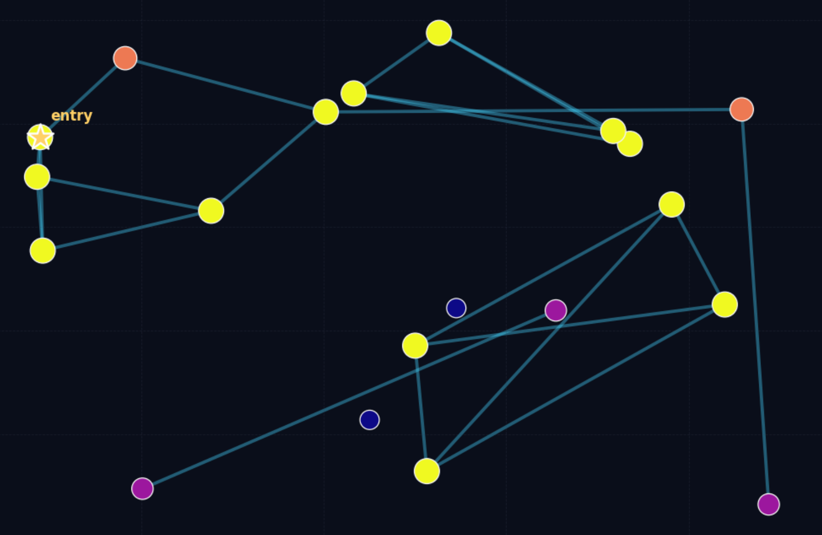
The figure above visually shows an unsatisfactory proximity graph: the darker the dots, the worse the connectivity. Some dots can hardly find their own neighbors, so the search stage struggles to route to them.

Navigable Small World

To solve the problems above, the industry came up with two ideas:

1. Hybrid algorithms: before searching the adjacency graph, do a coarse ranking first to find a more suitable entry point, and then perform greedy search.
2. Navigable small world structures: control search complexity through good connectivity plus a cap on the maximum number of neighbors per node.

NSW (Navigable Small World) takes the second approach.

The NSW model was first proposed by J. Kleinberg in social experiments, used to study connections between people in society, that is, the famous six degrees of separation theory.

For K-NN graph algorithms specifically, all small-world networks that have logarithmic or polylogarithmic complexity at search time are called Navigable Small World Networks. There are many implementations, which are not covered here.

NSW represented state-of-the-art search performance on some datasets at the time, but because it is not strictly logarithmic in complexity, it underperforms on test sets such as low-dimensional vector spaces.

Hierarchical Navigable Small World

The NSW algorithm has two phases at search time:

Phase	Behavior
zoom-out	Randomly pick a low-degree vertex as the entry point. During search, prefer high-degree nodes until the average distance from a node to its neighbors exceeds the distance from that node to the query vector
zoom-in	After finding a suitable high-degree node, run greedy search until the best TopN is found

NSW has polylogarithmic complexity because the total number of distance computations is roughly proportional to "number of hops x average degree of the vertices passed through", and both the average number of hops and the average degree grow logarithmically with the data scale, so the overall complexity is polylogarithmic.

HNSW reduces query time complexity to logarithmic time by accelerating the zoom-out process.

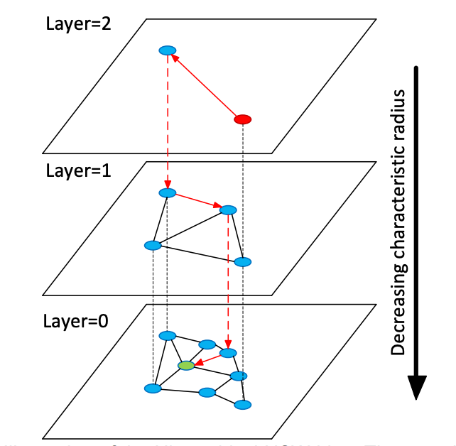
In HNSW, "hierarchy" means: the vertices in the NSW graph are layered according to the characteristic radius of their edges. The search flow is as follows:

1. Pick the entry point at the topmost layer to begin.
2. Run greedy search on the current layer to find the closest point on that layer.
3. Move down one layer and repeat the greedy search.
4. Continue until the bottom layer is reached, producing the final result.

Because the maximum number of connections per node is capped on every layer, the overall logarithmic time complexity is preserved.

To build the hierarchy, when each node is inserted, HNSW computes its layer l according to a geometric distribution, ensuring that there are not too many layers overall. HNSW does not require shuffling the data before ingestion (in NSW, shuffling is mandatory; otherwise the graph quality suffers), because the random layer assignment during indexing is itself a randomization step. This is also why HNSW supports true incremental updates.

HNSW In Apache Doris

Doris has supported building ANN indexes based on the HNSW algorithm since version 4.0.

Building an Index

There are two ways to create an ANN index:

Method	Trigger	Pros	Cons
Specify at table creation	Built synchronously when the segment is created during data ingestion	The index is available for query acceleration as soon as ingestion completes	Synchronous building slows down ingestion, and compaction rebuilds the index repeatedly
CREATE/BUILD INDEX	Built asynchronously after data ingestion	Does not affect ingestion speed and makes parameter tuning easier	ANN acceleration is unavailable while the index is being built

Method 1: Specify the Index at Table Creation

Suitable for stable scenarios where you know the index parameters and do not need frequent tuning.

CREATE TABLE sift_1M (
    id int NOT NULL,
    embedding array<float>  NOT NULL  COMMENT "",
    INDEX ann_index (embedding) USING ANN PROPERTIES(
        "index_type"="hnsw",
        "metric_type"="l2_distance",
        "dim"="128"
    )
) ENGINE=OLAP
DUPLICATE KEY(id) COMMENT "OLAP"
DISTRIBUTED BY HASH(id) BUCKETS 1
PROPERTIES (
    "replication_num" = "1"
);

INSERT INTO sift_1M
SELECT *
FROM S3(
    "uri" = "https://selectdb-customers-tools-bj.oss-cn-beijing.aliyuncs.com/sift_database.tsv",
    "format" = "csv");

Method 2: CREATE / BUILD INDEX

Suitable for scenarios that require flexible tuning and are sensitive to ingestion performance.

Step 1: Create the table (without an index) and ingest data.

CREATE TABLE sift_1M (
    id int NOT NULL,
    embedding array<float>  NOT NULL  COMMENT ""
) ENGINE=OLAP
DUPLICATE KEY(id) COMMENT "OLAP"
DISTRIBUTED BY HASH(id) BUCKETS 1
PROPERTIES (
    "replication_num" = "1"
);

INSERT INTO sift_1M
SELECT *
FROM S3(
    "uri" = "https://selectdb-customers-tools-bj.oss-cn-beijing.aliyuncs.com/sift_database.tsv",
    "format" = "csv");

Step 2: Add the index definition with CREATE INDEX. At this point only the index definition exists; the index has not yet been built on the existing data.

CREATE INDEX idx_test_ann ON sift_1M (`embedding`) USING ANN PROPERTIES (
    "index_type"="hnsw",
    "metric_type"="l2_distance",
    "dim"="128"
);

SHOW DATA ALL FROM sift_1M;

Example output:

+-----------+-----------+--------------+----------+----------------+---------------+----------------+-----------------+----------------+-----------------+
| TableName | IndexName | ReplicaCount | RowCount | LocalTotalSize | LocalDataSize | LocalIndexSize | RemoteTotalSize | RemoteDataSize | RemoteIndexSize |
+-----------+-----------+--------------+----------+----------------+---------------+----------------+-----------------+----------------+-----------------+
| sift_1M   | sift_1M   | 1            | 1000000  | 170.001 MB     | 170.001 MB    | 0.000          | 0.000           | 0.000          | 0.000           |
|           | Total     | 1            |          | 170.001 MB     | 170.001 MB    | 0.000          | 0.000           | 0.000          | 0.000           |
+-----------+-----------+--------------+----------+----------------+---------------+----------------+-----------------+----------------+-----------------+
2 rows in set (0.01 sec)

Step 3: Trigger the actual build with BUILD INDEX.

BUILD INDEX idx_test_ann ON sift_1M;

BUILD INDEX runs asynchronously. You can check the task status with SHOW BUILD INDEX:

SHOW BUILD INDEX WHERE TableName = "sift_1M";

Example output:

+---------------+-----------+---------------+------------------------------------------------------------------------------------------------------------------------------------+-------------------------+-------------------------+---------------+----------+------+----------+
| JobId         | TableName | PartitionName | AlterInvertedIndexes                                                                                                               | CreateTime              | FinishTime              | TransactionId | State    | Msg  | Progress |
+---------------+-----------+---------------+------------------------------------------------------------------------------------------------------------------------------------+-------------------------+-------------------------+---------------+----------+------+----------+
| 1763603913428 | sift_1M   | sift_1M       | [ADD INDEX idx_test_ann (`embedding`) USING ANN PROPERTIES("dim" = "128", "index_type" = "hnsw", "metric_type" = "l2_distance")],  | 2025-11-20 11:14:55.253 | 2025-11-20 11:15:10.622 | 126128        | FINISHED |      | NULL     |
+---------------+-----------+---------------+------------------------------------------------------------------------------------------------------------------------------------+-------------------------+-------------------------+---------------+----------+------+----------+

DROP INDEX

During the tuning phase, you may need to test different parameter combinations. Use DROP INDEX to manage indexes flexibly:

ALTER TABLE sift_1M DROP INDEX idx_test_ann;

Running Queries

The ANN index supports acceleration for both TopN search and Range search.

When the vector column has a high dimensionality, the string that describes the query vector itself introduces additional parsing overhead. In production environments (especially under high concurrency), do not run vector searches with raw SQL directly. Instead, use a prepared statement to perform SQL parsing in advance.

Doris officially provides a vector search Python library. It encapsulates the operations needed to use prepared statements and integrates a data conversion pipeline that turns query results directly into a pandas DataFrame, making it convenient to develop AI applications on top of Doris.

from doris_vector_search import DorisVectorClient, AuthOptions

auth = AuthOptions(
    host="localhost",
    query_port=9030,
    user="root",
    password="",
)

client = DorisVectorClient(database="demo", auth_options=auth)

tbl = client.open_table("sift_1M")

query = [0.1] * 128  # Example 128-dimensional vector

# SELECT id FROM sift_1M ORDER BY l2_distance_approximate(embedding, query) LIMIT 10;
result = tbl.search(query, metric_type="l2_distance").limit(10).select(["id"]).to_pandas()

print(result)

Example execution result:

       id
0  123911
1   11743
2  108584
3  123739
4   73311
5  124746
6  620941
7  124493
8  177392
9  153178

Recall Optimization

The most important metric in vector search is recall. Any performance number is meaningful only when a certain recall level is met. The factors that affect recall are mainly:

1. HNSW indexing-stage parameters (max_degree, ef_construction) and query-stage parameters (ef_search)
2. Index vector quantization
3. The size and number of segments

This section discusses items 1 and 3. Vector quantization is covered in other articles.

Index Hyperparameters

The HNSW index organizes vectors as a hierarchical graph. The build phase mainly consists of three steps:

1. Multi-layer random layer assignment: each vector is randomly assigned to multiple layers. Higher layers are sparser and are used for fast navigation.
2. Search candidate neighbors with ef_construction: on each layer, HNSW performs a breadth-first local search using a candidate queue with maximum length ef_construction. A larger value yields more accurate neighbors and a better graph structure, but takes longer to build.
3. Limit connections with max_degree: the number of neighbors per node is limited by max_degree, preventing the graph from becoming too dense.

The query phase consists of two steps:

1. High-layer greedy search (Coarse search): starting from the entry point, greedy search runs from the top down on the upper layers and quickly approaches the target region.
2. Bottom-layer breadth search (Fine search): on layer 0, a more thorough neighborhood expansion is performed using a candidate queue with maximum length ef_search.

The roles and trade-offs of the three core parameters:

Parameter	Role	Default	Effect of Increasing
max_degree	Number of bidirectional edges stored per node in the graph	32	Recall increases, memory usage increases, query performance decreases
ef_construction	Maximum length of the candidate queue during the indexing phase	40	Graph quality improves, recall increases, build time grows
ef_search	Maximum length of the candidate queue during the query phase	32	Recall increases, the number of distance computations grows, and query latency and CPU cost rise

The table below shows measured results on the SIFT_1M dataset:

max_degree	ef_construction	ef_search	recall@1	recall@100
32	80	32	0.955	0.75335
32	80	64	0.98	0.88015
32	80	96	0.995	0.9328
32	120	32	0.96	0.7736
32	120	64	0.975	0.89865
32	120	96	0.99	0.94575
32	160	32	0.955	0.78745
32	160	64	0.98	0.9097
32	160	96	0.995	0.95485
48	80	32	0.985	0.85895
48	80	64	0.99	0.9453
48	80	96	1	0.97325
48	120	32	0.97	0.78335
48	120	64	1	0.9089
48	120	96	1	0.95325
48	160	32	0.975	0.79745
48	160	64	0.995	0.9192
48	160	96	0.995	0.9601
64	80	32	1	0.9026
64	80	64	1	0.97025
64	80	96	1	0.9862
64	120	32	0.985	0.8548
64	120	64	0.99	0.94755
64	120	96	0.995	0.97645
64	160	32	0.97	0.80585
64	160	64	0.99	0.91925
64	160	96	0.995	0.96165

As you can see, multiple parameter combinations can reach the same recall level. For example, when targeting recall@100 > 95%, the qualifying combinations include:

max_degree	ef_construction	ef_search	recall@1	recall@100
32	160	96	0.995	0.95485
48	80	96	1	0.97325
48	120	96	1	0.95325
48	160	96	0.995	0.9601
64	80	64	1	0.97025
64	80	96	1	0.9862
64	120	96	0.995	0.97645
64	160	96	0.995	0.96165

Practical method for selecting hyperparameters:

1. Create a table table_multi_index with no indexes that has multiple vector columns (2 to 3 vector columns).
2. Ingest the data into this table via Stream Load or other methods.
3. Build indexes on all vector columns with CREATE INDEX and BUILD INDEX, using a different parameter combination on each column.
4. After the indexes are built, compute recall on each column separately and pick the most suitable hyperparameter combination.

Number of Rows Covered by an Index

Data in a Doris internal table is organized hierarchically:

Level	Meaning
Table	The top-level concept
Tablet	The basic unit of data migration and rebalancing. Table data is evenly distributed across N tablets by the bucket key
Rowset	The basic unit of version management. Each ingestion or compaction adds a new rowset under the tablet
Segment	The actual files that store data

As with the inverted index, the vector index also operates at segment granularity. Segment size is determined by the BE configurations write_buffer_size and vertical_compaction_max_segment_size. During ingestion and compaction, when a memtable reaches a certain size it is flushed into a segment file, and a vector index is built for that segment (one index per index column).

According to the search and build mechanism of HNSW, for a given set of index parameters, the data range that can be effectively covered is limited. Once the data volume exceeds the threshold, the recall can no longer meet the requirement.

Empirical values for some hyperparameters and the number of rows per segment they can cover:

max_degree	ef_construction	ef_search	num_segment	recall@100
32	160	96	1M	0.95485
48	80	96	1M	0.97325
32	160	32	3M	0.66983
128	512	128	3M	0.9931

Run SHOW TABLETS FROM <table> to view the compaction state of the table. Click the corresponding URL to view the number of segments.

Effect of Compaction on Recall

Compaction sometimes produces larger segments, causing the original index hyperparameters to lose coverage on the new, larger segments.

Best practice: trigger a FULL COMPACTION before running BUILD INDEX. Building the index on fully compacted segments brings two benefits at once:

• Stable recall
• Less write amplification introduced by index building

Query Performance

Cold Loading of Index Files

The Doris ANN index is implemented based on Meta's open-source faiss. An HNSW index can accelerate queries only after the entire graph structure has been loaded into memory.

Before high-concurrency queries, run a cold query first to warm up the index files of the involved segments into memory. Otherwise, query performance drops significantly.

Memory Footprint and Performance

An HNSW index (without quantization compression) takes about 1.2x the memory of the vectors it indexes.

For example, for a 128-dimensional, 1M dataset, an HNSW FLAT index needs about 128 x 4 x 1,000,000 x 1.3 ~= 650 MB.

Estimated memory at different scales:

dim	rows	Estimated memory
128	1M	650 MB
768	10M	48 GB
768	100M	110 GB

To ensure query performance, BE nodes need to be configured with enough memory. Otherwise, frequent index I/O causes significant degradation in query performance.

Benchmark

Test hardware: a 16C 64GB machine. Test framework: VectorDBBench. Load client: another 16C machine.

The typical deployment mode for a Doris production cluster is separate deployment of FE and BE (which requires two 16C 64GB machines). The table below also lists the test results for mixed deployment of FE and BE alongside the typical deployment.

Performance768D1M

Test command:

NUM_PER_BATCH=1000000 python3.11 -m vectordbbench doris --host 127.0.0.1 --port 9030 --case-type Performance768D1M --db-name Performance768D1M --search-concurrent --search-serial --num-concurrency 10,40,80 --stream-load-rows-per-batch 500000 --index-prop max_degree=128,ef_construction=512 --session-var hnsw_ef_search=128

Comparison of test results:

	Doris (FE/BE separated)	Doris (FE/BE mixed)
Index prop	max_degree=128, ef_construction=512, hnsw_ef_search=128	max_degree=128, ef_construction=512, hnsw_ef_search=156
Recall@100	0.9931	0.9929
Concurrency (Client)	10, 40, 80	10, 40, 80
Result QPS	163.1567 (10) 606.6832 (40) 859.3842 (80)	162.3002 (10) 542.3488 (40) 607.7951 (80)
Avg Latency (s)	0.06123 (10) 0.06579 (40) 0.09281 (80)	0.06154 (10) 0.07351 (40) 0.13093 (80)
P95 Latency (s)	0.06560 (10) 0.07747 (40) 0.12967 (80)	0.06726 (10) 0.08789 (40) 0.18719 (80)
P99 Latency (s)	0.06889 (10) 0.08618 (40) 0.14605 (80)	0.06154 (10) 0.07351 (40) 0.13093 (80)