IVF: Accelerating Vector Search in Apache Doris with IVF Indexes
One-sentence definition: IVF (Inverted File Index) is an approximate nearest neighbor (ANN) index that partitions the vector space through clustering to narrow the search range. It has been natively supported since Apache Doris 4.x.
This article answers the following questions:
- What is the IVF index? Why does it accelerate vector retrieval?
- How do you create, build, and drop an IVF index in Apache Doris?
- How do you choose key parameters such as
nlistandnprobeto balance recall and performance? - What factors affect recall? How do you avoid performance degradation?
Quick Navigation
| Your goal | Jump to |
|---|---|
| Understand the basic principles of IVF | What Is the IVF Index |
| Create and use an IVF index | Using IVF in Apache Doris |
| Tune recall | Recall Optimization |
| Troubleshoot query performance | Query Performance |
| Reproduce performance benchmarks | Benchmark |
| Common questions | FAQ |
What Is the IVF Index
From Inverted Indexes to Vector Inverted Indexes
The term IVF (Inverted File) originates from the field of information retrieval. Take text retrieval as an example:
-
Forward index: Each document maintains a list of words. The query must scan all documents.
Document Words Document 1 the, cow, says, moo Document 2 the, cat, and, the, hat Document 3 the, dish, ran, away, with, the, spoon -
Inverted index: Each word maintains a list of "documents that contain this word." The query only needs to scan the relevant lists.
Word Documents the Document 1, Document 3, Document 4, Document 5, Document 7 cow Document 2, Document 3, Document 4 says Document 5 moo Document 7
Today, text is usually represented as vector embeddings. IVF borrows the inverted-index idea: cluster centroids act as the "dictionary," and each centroid maintains a list of "vectors that belong to this cluster." A query only needs to inspect a small number of selected clusters.
Why IVF Accelerates Vector Search
When a dataset grows to millions or billions of vectors, exact kNN search (computing the distance between the query vector and every vector in the database) is equivalent to a large-scale matrix multiplication, and the computational cost becomes unacceptable.
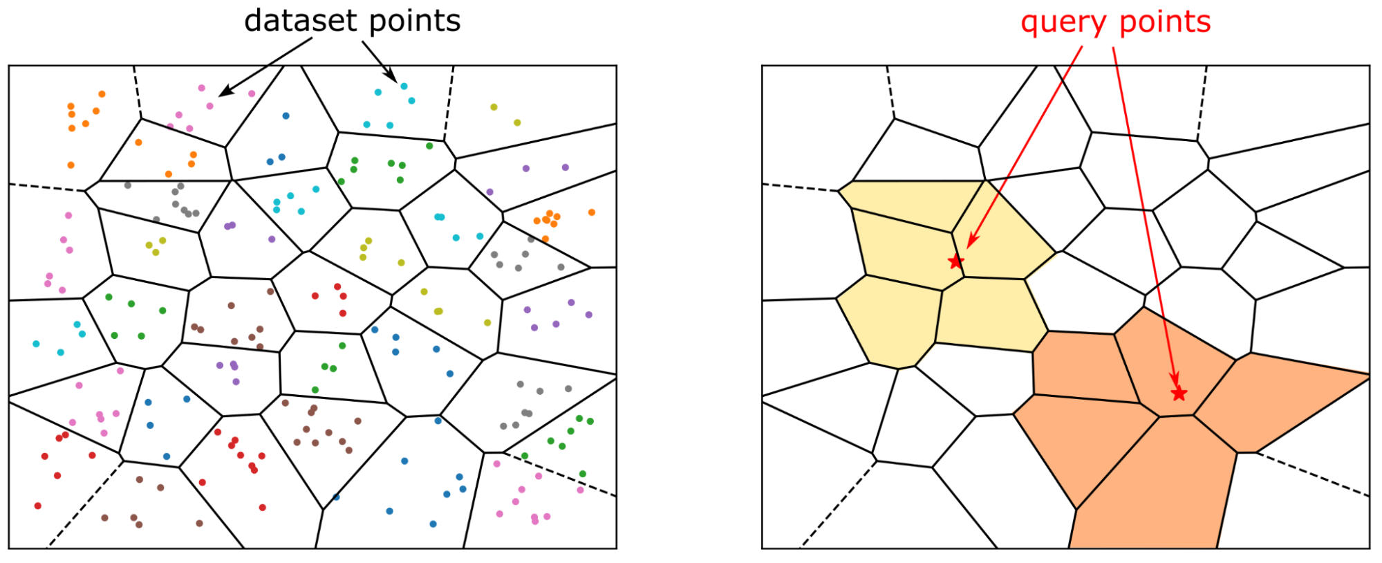
Approximate nearest neighbor (ANN) search trades a small amount of accuracy for an order-of-magnitude speedup. IVF is one of the most widely used and effective ANN methods in industry. Its core idea is "divide and conquer":
- Partition the entire vector dataset into multiple clusters, each represented by a centroid.
- At query time, first identify the small number of clusters whose centroids are closest to the query vector, search only within these clusters, and skip the rest of the data.
Using IVF in Apache Doris
Apache Doris has supported IVF-based ANN indexes since version 4.x. The index type is fixed as ANN, and the IVF algorithm is selected by specifying index_type=ivf.
Index Building Approaches
There are two ways to create an ANN index, suitable for different scenarios:
| Approach | Build timing | Pros | Cons | Applicable scenarios |
|---|---|---|---|---|
| Define index at table creation | Built synchronously during data ingestion | Queries are accelerated as soon as data is written | Slows down writes; Compaction may trigger index rebuilds, wasting resources | Production environments where index parameters are already finalized |
CREATE INDEX + BUILD INDEX | Built asynchronously after data is loaded | Does not affect ingestion; convenient for parameter tuning | No acceleration during the build period | Parameter-tuning phase, initialization of very large tables |
Approach 1: Define the Index at Table Creation
CREATE TABLE sift_1M (
  id int NOT NULL,
  embedding array<float>  NOT NULL  COMMENT "",
  INDEX ann_index (embedding) USING ANN PROPERTIES(
      "index_type"="ivf",
      "metric_type"="l2_distance",
      "dim"="128",
      "nlist"="1024"
  )
) ENGINE=OLAP
DUPLICATE KEY(id) COMMENT "OLAP"
DISTRIBUTED BY HASH(id) BUCKETS 1
PROPERTIES (
  "replication_num" = "1"
);

INSERT INTO sift_1M
SELECT *
FROM S3(
  "uri" = "https://selectdb-customers-tools-bj.oss-cn-beijing.aliyuncs.com/sift_database.tsv",
  "format" = "csv");
Approach 2: CREATE INDEX + BUILD INDEX
Step 1: Create the table (without the index) and load the data.
CREATE TABLE sift_1M (
  id int NOT NULL,
  embedding array<float>  NOT NULL  COMMENT ""
) ENGINE=OLAP
DUPLICATE KEY(id) COMMENT "OLAP"
DISTRIBUTED BY HASH(id) BUCKETS 1
PROPERTIES (
  "replication_num" = "1"
);

INSERT INTO sift_1M
SELECT *
FROM S3(
  "uri" = "https://selectdb-customers-tools-bj.oss-cn-beijing.aliyuncs.com/sift_database.tsv",
  "format" = "csv");
Step 2: Run CREATE INDEX to add the index definition. At this point, only the index metadata is registered; the index has not yet been built on the existing data.
CREATE INDEX idx_test_ann ON sift_1M (`embedding`) USING ANN PROPERTIES (
  "index_type"="ivf",
  "metric_type"="l2_distance",
  "dim"="128",
  "nlist"="1024"
);

SHOW DATA ALL FROM sift_1M;
Expected output (LocalIndexSize is still 0):
+-----------+-----------+--------------+----------+----------------+---------------+----------------+-----------------+----------------+-----------------+
| TableName | IndexName | ReplicaCount | RowCount | LocalTotalSize | LocalDataSize | LocalIndexSize | RemoteTotalSize | RemoteDataSize | RemoteIndexSize |
+-----------+-----------+--------------+----------+----------------+---------------+----------------+-----------------+----------------+-----------------+
| sift_1M   | sift_1M   | 10           | 1000000  | 170.093 MB     | 170.093 MB    | 0.000          | 0.000           | 0.000          | 0.000           |
|           | Total     | 10           |          | 170.093 MB     | 170.093 MB    | 0.000          | 0.000           | 0.000          | 0.000           |
+-----------+-----------+--------------+----------+----------------+---------------+----------------+-----------------+----------------+-----------------+
Step 3: Run BUILD INDEX to build the index on the existing data. This task runs asynchronously.
BUILD INDEX idx_test_ann ON sift_1M;
Step 4: Check the task status with SHOW BUILD INDEX.
SHOW BUILD INDEX WHERE TableName = "sift_1M";
After the task finishes, check the data size again. The index size (LocalIndexSize) has been generated:
+---------------+-----------+---------------+-----------------------------------------------------------------------------------------------------------------------------------------------------+-------------------------+-------------------------+---------------+----------+------+----------+
| JobId         | TableName | PartitionName | AlterInvertedIndexes                                                                                                                                | CreateTime              | FinishTime              | TransactionId | State    | Msg  | Progress |
+---------------+-----------+---------------+-----------------------------------------------------------------------------------------------------------------------------------------------------+-------------------------+-------------------------+---------------+----------+------+----------+
| 1764392359610 | sift_1M   | sift_1M       | [ADD INDEX idx_test_ann (`embedding`) USING ANN PROPERTIES("dim" = "128", "index_type" = "ivf", "metric_type" = "l2_distance", "nlist" = "1024")],  | 2025-12-01 14:18:22.360 | 2025-12-01 14:18:27.885 | 5036          | FINISHED |      | NULL     |
+---------------+-----------+---------------+-----------------------------------------------------------------------------------------------------------------------------------------------------+-------------------------+-------------------------+---------------+----------+------+----------+

mysql> SHOW DATA ALL FROM sift_1M;
+-----------+-----------+--------------+----------+----------------+---------------+----------------+-----------------+----------------+-----------------+
| TableName | IndexName | ReplicaCount | RowCount | LocalTotalSize | LocalDataSize | LocalIndexSize | RemoteTotalSize | RemoteDataSize | RemoteIndexSize |
+-----------+-----------+--------------+----------+----------------+---------------+----------------+-----------------+----------------+-----------------+
| sift_1M   | sift_1M   | 10           | 1000000  | 671.084 MB     | 170.093 MB    | 500.991 MB     | 0.000           | 0.000          | 0.000           |
|           | Total     | 10           |          | 671.084 MB     | 170.093 MB    | 500.991 MB     | 0.000           | 0.000          | 0.000           |
+-----------+-----------+--------------+----------+----------------+---------------+----------------+-----------------+----------------+-----------------+
Dropping the Index
During parameter tuning, you often need to test different parameter combinations to ensure recall. Use DROP INDEX to manage indexes flexibly:
ALTER TABLE sift_1M DROP INDEX idx_test_ann;
Running Vector Queries
ANN indexes accelerate both TopN search and range search.
Production best practice: The string representation of high-dimensional vectors introduces extra overhead during SQL parsing, so using raw SQL directly is not recommended in high-concurrency scenarios. Two optimization options are recommended:
- Use a Prepare Statement to pre-parse the SQL.
- Use the official Doris vector search Python library. This library wraps Prepare Statement calls and converts query results directly into a pandas DataFrame, which is convenient for AI application development.
Example code:
from doris_vector_search import DorisVectorClient, AuthOptions

auth = AuthOptions(
    host="127.0.0.1",
    query_port=9030,
    user="root",
    password="",
)

client = DorisVectorClient(database="test", auth_options=auth)

tbl = client.open_table("sift_1M")

query = [0.1] * 128  # Example 128-dimensional vector

# SELECT id FROM sift_1M ORDER BY l2_distance_approximate(embedding, query) LIMIT 10;
result = tbl.search(query, metric_type="l2_distance").limit(10).select(["id"]).to_pandas()

print(result)
Expected output:
       id
0  123911
1  926855
2  123739
3   73311
4  124493
5  153178
6  126138
7  123740
8  125741
9  124048
Recall Optimization
The core metric of vector search is recall. Any performance figure is meaningful only when recall is acceptable. The main factors that affect recall are:
- IVF index parameters (
nlist) and query parameters (nprobe) - Vector quantization in the index
- The size and number of Segments
This section discusses items 1 and 3. Vector quantization is covered in other documents.
Index Hyperparameters: nlist and nprobe
IVF uses key parameters during index building and at query time:
Index building phase:
- Clustering: Use a clustering algorithm (such as k-means) to partition the vectors into
nlistclusters, then compute and store the centroid of each cluster. - Vector assignment: Assign each vector to the cluster whose centroid is closest to it, and add the vector to the corresponding inverted list.
Query phase:
- Cluster selection: Compute the distance from the query vector to all
nlistcentroids and pick the closestnprobeclusters. - Within-cluster exhaustive search: Compare vectors one by one inside the selected
nprobeclusters to find the nearest neighbors.
| Parameter | Purpose | Effect | Doris default |
|---|---|---|---|
nlist | Number of clusters (inverted lists) | A larger value gives finer granularity and faster search, but increases clustering cost and makes neighbors more likely to be scattered across different clusters | 1024 |
nprobe | Number of clusters probed at query time | A larger value gives higher recall and higher latency; a smaller value is faster but more likely to miss results | 64 |
Measured results on the SIFT_1M dataset:
| nlist | nprobe | recall@100 |
|---|---|---|
| 1024 | 64 | 0.9542 |
| 1024 | 32 | 0.9034 |
| 1024 | 16 | 0.8299 |
| 1024 | 8 | 0.7337 |
| 512 | 32 | 0.9384 |
| 512 | 16 | 0.8763 |
| 512 | 8 | 0.7869 |
Hyperparameter Selection in Practice
Although the exact optimal parameters cannot be determined in advance, you can choose them systematically as follows:
- Create a temporary table
table_multi_indexwithout indexes that contains 2 to 3 vector columns. - Load data into this table through Stream Load or another method.
- Run
CREATE INDEXandBUILD INDEXwith different parameters on each vector column. - Compare the recall of each column and pick the parameter combination that fits best.
Example:
ALTER TABLE tbl DROP INDEX idx_embedding;
CREATE INDEX idx_embedding ON tbl (`embedding`) USING ANN PROPERTIES (
  "index_type"="ivf",
  "metric_type"="inner_product",
  "dim"="768",
  "nlist"="1024"
);
BUILD INDEX idx_embedding ON tbl;
Number of Rows Covered by the Index
Data in a Doris internal table is organized in the following hierarchy:
- Table to Tablet: Distributed evenly across N Tablets by the bucket key (the basic unit of data migration and rebalancing).
- Tablet to Rowset: Each load or Compaction adds a new Rowset (the unit of version management).
- Rowset to Segment: The actual data is stored in Segment files.
Like inverted indexes, vector indexes operate at Segment granularity. The Segment size is controlled by the BE configuration items write_buffer_size and vertical_compaction_max_segment_size. During loading or Compaction, when the memtable accumulates to a certain size, it is flushed to a Segment file, and a vector index is built for that Segment (multiple index columns produce multiple indexes).
Each combination of IVF index parameters can effectively cover only a limited amount of data. When the number of rows in a Segment exceeds a threshold, recall drops.
Tip: Use
SHOW TABLETS FROM <table>to check the Compaction status of a table. Open the corresponding URL to see the number of Segments.
Effect of Compaction on Recall
Compaction merges multiple small Segments into larger ones, which makes index parameters that were tuned for smaller data sizes ineffective and reduces recall.
Best practice: Trigger a FULL COMPACTION before running BUILD INDEX. Building the index on fully merged Segments has two benefits:
- Recall stays stable.
- Write amplification introduced by index building is reduced.
Query Performance
Cold Loading of Index Files
The Doris ANN index is implemented on top of Meta's open-source faiss. An IVF index must be fully loaded into memory before it can accelerate queries.
Best practice: Run a cold query before high-concurrency queries to ensure that all relevant Segment index files have been loaded. Otherwise, performance on the first query degrades significantly.
Memory Footprint and Performance
An IVF index without quantization compression occupies about 1.02 times the memory of the vectors it indexes.
For example, the memory footprint of an IVF FLAT index for a 128-dimensional, 1M-row dataset is approximately:
128 * 4 * 1,000,000 * 1.02 ≈ 500 MB
Reference values:
| dim | rows | Estimated memory |
|---|---|---|
| 128 | 1M | 500 MB |
| 768 | 1M | 2.9 GB |
To guarantee query performance, the BE must have enough memory to hold the entire index. Otherwise, frequent IO on index files causes severe query performance degradation.
Benchmark
Deployment recommendation: Benchmarks should mimic a production environment. Deploy FE and BE separately, and run the client on a separate machine.
Test framework: VectorDBBench.
Performance768D1M
Benchmark commands:
# load
NUM_PER_BATCH=1000000 python3 -m vectordbbench doris --host 127.0.0.1 --port 9030 --case-type Performance768D1M --db-name Performance768D1M --stream-load-rows-per-batch 500000 --index-prop index_type=ivf,nlist=1024 --skip-search-serial --skip-search-concurrent

# search
NUM_PER_BATCH=1000000 python3 -m vectordbbench doris --host 127.0.0.1 --port 9030 --case-type Performance768D1M --db-name Performance768D1M --search-concurrent --search-serial --num-concurrency 10,40,80 --stream-load-rows-per-batch 500000 --index-prop index_type=ivf,nlist=1024 --session-var ivf_nprobe=64 --skip-load --skip-drop-old
FAQ
Q1: How should you choose between IVF and HNSW? IVF is suitable for large-scale scenarios that have sufficient memory and need to balance build cost with query latency. HNSW has an advantage in query latency but a higher memory footprint. See the HNSW documentation for details.
Q2: Why is recall still low after BUILD INDEX?
Common causes include: nprobe is set too low, Segments are too large so the index does not cover them well, or FULL COMPACTION was not run before BUILD. See Recall Optimization.
Q3: Why run a cold query before high-concurrency queries? The IVF index must be fully loaded into memory to accelerate queries. The cold query warms the cache by loading the index from disk into memory, which avoids performance degradation on the first online query.
Q4: Does the default nlist value of 1024 need to be adjusted?
Doris defaults to nlist=1024 and nprobe=64, which work for most medium-sized datasets. Adjust based on your actual data size and recall requirements following Hyperparameter Selection in Practice.
Q5: Does DROP INDEX release memory immediately?
DROP INDEX removes the index definition, and the index files are cleaned up afterwards. During parameter tuning, use it together with the CREATE INDEX and BUILD INDEX workflow.
Troubleshooting
| Symptom | Possible cause | Solution |
|---|---|---|
| Recall is significantly lower than expected | nprobe is too low / Segments are too large / FULL COMPACTION was not run | Increase nprobe; run FULL COMPACTION before BUILD; adjust nlist |
| First query has very high latency, subsequent queries are normal | The index has not yet been loaded into memory (cold load) | Run a cold query to warm up before high-concurrency queries |
| BE memory is tight and query performance degrades | The index does not fully reside in memory, causing frequent IO | Expand BE memory; consider using quantization compression to reduce memory usage |
BUILD INDEX does not finish for a long time | The task is asynchronous and the data volume is large | Check progress with SHOW BUILD INDEX WHERE TableName = "<tbl>" |
| Data ingestion becomes slow | The index is built synchronously at table creation | Switch to the CREATE INDEX + BUILD INDEX approach to build asynchronously |