HNSW and How to use it in Apaceh Doris

HNSW (Malkov & Yashunin, 2016) has become the de facto standard for high‑performance online vector search thanks to its ability to achieve high recall and low latency with relatively modest resource consumption. Since Apache Doris 4.x, an ANN index based on HNSW has been supported. This document walks through the HNSW algorithm, key parameters, and engineering practices, and explains how to build and tune HNSW‑based ANN indexes in production Doris clusters.

Before HNSW

The HNSW (Hierarchical Navigable Small World) algorithm was proposed in the paper Efficient and robust approximate nearest neighbor search using Hierarchical Navigable Small World graphs. Before HNSW, many algorithms had already been proposed for approximate k‑NN search, but each came with its own limitations.

Proximate Graph

The basic idea of this family of algorithms is to start from an entry point in the graph (which can be a random vertex or a vertex chosen by some heuristic), and then iteratively traverse the graph. At each iteration, the algorithm computes the distance between the query vector and all neighbors of the current node, picks the closest neighbor as the new base node for the next iteration, and continuously maintains the current best candidate set. When certain stopping conditions are met—such as no closer node being found in the last iteration—the algorithm terminates and the top K nearest nodes in the candidate set are returned as the final result.

These proximity‑graph algorithms can be seen as approximations of a Delaunay graph, because a Delaunay graph has an important property: a greedy search always finds the nearest neighbor.

However, this family of algorithms has two main issues:

1. As the dataset grows, the number of iterations in the routing phase increases roughly following a power‑law.
2. It is difficult to build a high‑quality proximity graph; local clusters and poor global connectivity are very common.

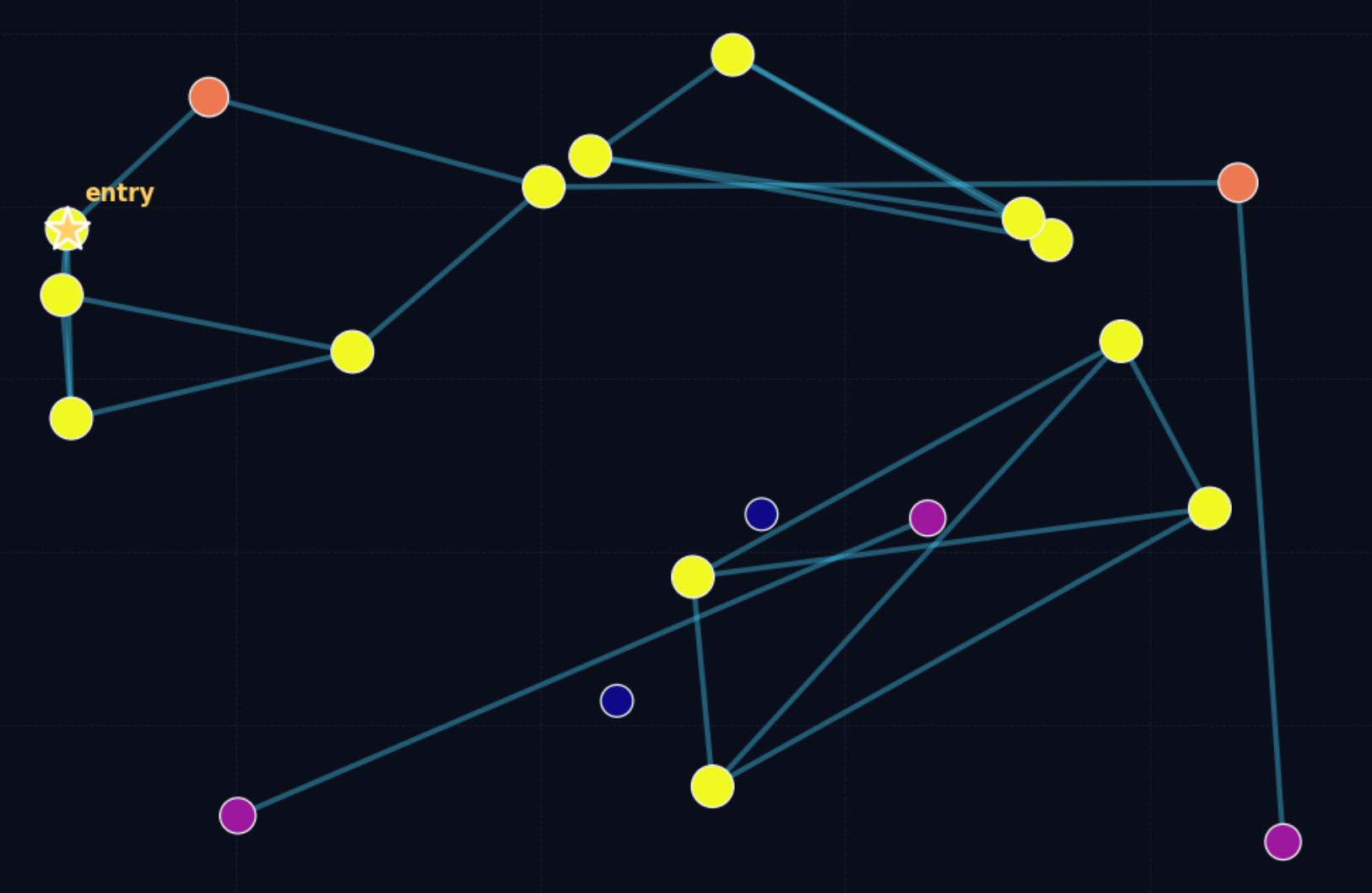
The figure above intuitively shows the shape of a problematic proximity graph. Darker points represent nodes with poorer connectivity; some nodes barely have any neighbors at all, which makes them very hard to reach during search.

Navigable Small World

To address the above issues, there are two main ideas:

1. Hybrid approaches: perform a coarse‑grained search first to find a better entry point, then run a greedy search on the proximity graph.
2. Use a navigable small‑world structure that maintains good connectivity while limiting each node’s maximum degree to control search complexity.

NSW (Navigable Small World) adopts the second idea.

The NSW model was first proposed in J. Kleinberg as part of a social experiment to study how people are connected in society. You might have heard of the small‑world experiment / six degrees of separation.

For k‑NN graph algorithms, any small‑world network that achieves logarithmic or polylogarithmic search complexity is often called a Navigable Small World Network. There are many concrete implementations, which we will not detail here.

On some datasets, NSW represented state‑of‑the‑art search performance at the time. However, because NSW does not have strictly logarithmic complexity, its performance can be suboptimal in certain benchmarks, especially on low‑dimensional vector spaces.

Hierarchical Navigable Small World

The NSW search process can be viewed as consisting of two phases: zoom‑out and zoom‑in.

• zoom-out: Start from a randomly chosen low‑degree vertex and search while preferring nodes with higher degrees, until the average distance to neighbors exceeds the distance from the current node to the query.
• zoom-in: Once a sufficiently “high” node under those conditions is found, perform greedy search to obtain the final Top‑N neighbors.

The reason NSW achieves polylogarithmic complexity is that the total number of distance evaluations is roughly proportional to the product of the number of jumps made during search and the average degree of the visited nodes. Both the number of jumps and the average degree grow approximately logarithmically with the data size, which leads to an overall polylogarithmic complexity.

HNSW reduces the query time complexity to logarithmic by accelerating the zoom‑out phase.

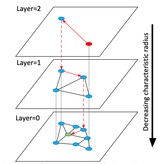
More concretely, the “hierarchical” structure in HNSW is obtained by splitting the NSW graph into multiple layers based on the characteristic radius (typical edge length) of nodes.

During search, HNSW chooses the top‑layer node as the entry point and performs greedy search layer by layer. Once the nearest node is found at the current layer, the search descends to the next layer and repeats the process until reaching the bottom layer. The maximum degree of nodes in each layer is capped, which helps keep the overall time complexity logarithmic.

To build this layered structure, HNSW assigns each node a level l according to a geometric distribution, ensuring that the structure does not grow too tall. HNSW also does not require shuffling the data before indexing (while NSW does, otherwise the graph quality suffers) because the random level assignment itself provides sufficient randomness. This design enables efficient incremental updates in HNSW.

HNSW in Apache Doris

Apache Doris supports building HNSW‑based ANN indexes starting from version 4.0.

Index Construction

The index type used here is ANN. There are two ways to create an ANN index: you can define it when creating the table, or you can use the CREATE/BUILD INDEX syntax. The two approaches differ in how and when the index is built, and therefore fit different scenarios.

Approach 1: define an ANN index on a vector column when creating the table. As data is loaded, an ANN index is built for each segment as it is created. The advantage is that once data loading completes, the index is already built and queries can immediately use it for acceleration. The downside is that synchronous index building slows down data ingestion and may cause extra index rebuilds during compaction, leading to some waste of resources.

CREATE TABLE sift_1M (
  id int NOT NULL,
  embedding array<float>  NOT NULL  COMMENT "",
  INDEX ann_index (embedding) USING ANN PROPERTIES(
      "index_type"="hnsw",
      "metric_type"="l2_distance",
      "dim"="128"
  )
) ENGINE=OLAP
DUPLICATE KEY(id) COMMENT "OLAP"
DISTRIBUTED BY HASH(id) BUCKETS 1
PROPERTIES (
  "replication_num" = "1"
);

INSERT INTO sift_1M
SELECT *
FROM S3(
  "uri" = "https://selectdb-customers-tools-bj.oss-cn-beijing.aliyuncs.com/sift_database.tsv",
  "format" = "csv");

CREATE/BUILD INDEX

Approach 2: CREATE/BUILD INDEX.

CREATE TABLE sift_1M (
  id int NOT NULL,
  embedding array<float>  NOT NULL  COMMENT ""
) ENGINE=OLAP
DUPLICATE KEY(id) COMMENT "OLAP"
DISTRIBUTED BY HASH(id) BUCKETS 1
PROPERTIES (
  "replication_num" = "1"
);

INSERT INTO sift_1M
SELECT *
FROM S3(
  "uri" = "https://selectdb-customers-tools-bj.oss-cn-beijing.aliyuncs.com/sift_database.tsv",
  "format" = "csv");

After data is loaded, you can run CREATE INDEX. At this point the index is defined on the table, but no index is yet built for the existing data.

CREATE INDEX idx_test_ann ON sift_1M (`embedding`) USING ANN PROPERTIES (
  "index_type"="hnsw",
  "metric_type"="l2_distance",
  "dim"="128"
);

SHOW DATA ALL FROM sift_1M

+-----------+-----------+--------------+----------+----------------+---------------+----------------+-----------------+----------------+-----------------+
| TableName | IndexName | ReplicaCount | RowCount | LocalTotalSize | LocalDataSize | LocalIndexSize | RemoteTotalSize | RemoteDataSize | RemoteIndexSize |
+-----------+-----------+--------------+----------+----------------+---------------+----------------+-----------------+----------------+-----------------+
| sift_1M   | sift_1M   | 1            | 1000000  | 170.001 MB     | 170.001 MB    | 0.000          | 0.000           | 0.000          | 0.000           |
|           | Total     | 1            |          | 170.001 MB     | 170.001 MB    | 0.000          | 0.000           | 0.000          | 0.000           |
+-----------+-----------+--------------+----------+----------------+---------------+----------------+-----------------+----------------+-----------------+
2 rows in set (0.01 sec)

Then you can build the index using the BUILD INDEX statement:

BUILD INDEX idx_test_ann ON sift_1M;

BUILD INDEX is executed asynchronously. You can use SHOW BUILD INDEX (in some versions SHOW ALTER) to check the job status.

SHOW BUILD INDEX WHERE TableName = "sift_1M";

+---------------+-----------+---------------+------------------------------------------------------------------------------------------------------------------------------------+-------------------------+-------------------------+---------------+----------+------+----------+
| JobId         | TableName | PartitionName | AlterInvertedIndexes                                                                                                               | CreateTime              | FinishTime              | TransactionId | State    | Msg  | Progress |
+---------------+-----------+---------------+------------------------------------------------------------------------------------------------------------------------------------+-------------------------+-------------------------+---------------+----------+------+----------+
| 1763603913428 | sift_1M   | sift_1M       | [ADD INDEX idx_test_ann (`embedding`) USING ANN PROPERTIES("dim" = "128", "index_type" = "hnsw", "metric_type" = "l2_distance")],  | 2025-11-20 11:14:55.253 | 2025-11-20 11:15:10.622 | 126128        | FINISHED |      | NULL     |
+---------------+-----------+---------------+------------------------------------------------------------------------------------------------------------------------------------+-------------------------+-------------------------+---------------+----------+------+----------+

DROP INDEX

You can drop an unsuitable ANN index with ALTER TABLE sift_1M DROP INDEX idx_test_ann. Dropping and recreating indexes is common during hyperparameter tuning, when you need to test different parameter combinations to achieve the desired recall.

Querying

ANN indexes support both Top‑N search and range search.

When the vector column has high dimensionality, the literal representation of the query vector itself can incur extra parsing overhead. Therefore, directly embedding the full query vector into raw SQL is not recommended in production, especially under high concurrency. A better practice is to use prepared statements, which avoid repetitive SQL parsing.

We recommend using the doris-vector-search python library, which wraps the necessary operations for vector search in Doris based on prepared statements, and includes data conversion utilities that map Doris query results into Pandas DataFrames for convenient downstream AI application development.

from doris_vector_search import DorisVectorClient, AuthOptions

auth = AuthOptions(
    host="localhost",
    query_port=8030,
    user="root",
    password="",
)

client = DorisVectorClient(database="demo", auth_options=auth)

tbl = client.open_table("sift_1M")

query = [0.1] * 128  # Example 128-dimensional vector

# SELECT id FROM sift_1M ORDER BY l2_distance_approximate(embedding, query) LIMIT 10;
result = tbl.search(query, metric_type="l2_distance").limit(10).select(["id"]).to_pandas()

print(result)

Sample output:

       id
0  123911
1   11743
2  108584
3  123739
4   73311
5  124746
6  620941
7  124493
8  177392
9  153178

Recall Optimization

In vector search, recall is the most important metric; performance numbers only make sense under a given recall level. The main factors that affect recall are:

1. Index‑time parameters of HNSW (max_degree, ef_construction) and query‑time parameter (ef_search).
2. Vector quantization.
3. Segment size and the number of segments.

This article focuses on the impact of (1) and (3) on recall. Vector quantization will be covered in a separate document.

Index Hyperparameters

An HNSW index organizes vectors into a multi‑layer graph. During index construction, vectors are inserted one by one and connected with neighbors across layers. The process is roughly as follows:

1. Layer assignment: Each vector is randomly assigned a level following a geometric distribution. Higher‑level nodes are sparser and act as shortcuts for navigation.
2. Search for candidate neighbors using ef_construction: At each level, HNSW uses a candidate queue of maximum size ef_construction to perform a local search. Larger ef_construction values generally yield better neighbors and higher‑quality graphs (and thus higher recall), at the cost of longer index‑building time.
3. Limit connections using max_degree: The number of neighbors for each node is capped by max_degree, which prevents the graph from becoming too dense.

At query time:

1. Greedy search on upper layers (coarse search): Starting from the entry node on the highest layer, HNSW performs greedy search on the upper layers to quickly move into the vicinity of the query.
2. Breadth‑like search on the bottom layer using ef_search (fine search): On layer 0, HNSW uses a candidate queue of maximum size ef_search to expand neighbors more thoroughly.

In summary:

• max_degree defines the maximum number of (bidirectional) edges per node. It affects recall, memory usage, and query performance. Larger max_degree usually yields higher recall but slower queries.
• ef_construction defines the maximum length of the candidate queue during index construction. Larger values improve graph quality and recall, but increase index‑build time.
• ef_search defines the maximum length of the candidate queue during query. Larger values improve recall, but increase the number of distance computations, which raises query latency and CPU usage.

By default, Doris uses max_degree = 32, ef_construction = 40, and ef_search = 32.

The above is a qualitative analysis of these three hyperparameters. The following table shows empirical results on the SIFT_1M dataset:

max_degree	ef_construction	ef_search	recall_at_1	recall_at_100
32	80	32	0.955	0.75335
32	80	64	0.98	0.88015
32	80	96	0.995	0.9328
32	120	32	0.96	0.7736
32	120	64	0.975	0.89865
32	120	96	0.99	0.94575
32	160	32	0.955	0.78745
32	160	64	0.98	0.9097
32	160	96	0.995	0.95485
48	80	32	0.985	0.85895
48	80	64	0.99	0.9453
48	80	96	1	0.97325
48	120	32	0.97	0.78335
48	120	64	1	0.9089
48	120	96	1	0.95325
48	160	32	0.975	0.79745
48	160	64	0.995	0.9192
48	160	96	0.995	0.9601
64	80	32	1	0.9026
64	80	64	1	0.97025
64	80	96	1	0.9862
64	120	32	0.985	0.8548
64	120	64	0.99	0.94755
64	120	96	0.995	0.97645
64	160	32	0.97	0.80585
64	160	64	0.99	0.91925
64	160	96	0.995	0.96165

The results show that multiple hyperparameter combinations can reach similar recall levels. For example, suppose you want recall@100 > 0.95. The following combinations all meet the requirement:

max_degree	ef_construction	ef_search	recall_at_1	recall_at_100
32	160	96	0.995	0.95485
48	80	96	1	0.97325
48	120	96	1	0.95325
48	160	96	0.995	0.9601
64	80	64	1	0.97025
64	80	96	1	0.9862
64	120	96	0.995	0.97645
64	160	96	0.995	0.96165

It is hard to provide one single optimal setting in advance, but you can follow a practical workflow for hyperparameter selection:

1. Create a table table_multi_index without indexes. It can contain 2 or 3 vector columns.
2. Load data into table_multi_index using Stream Load or other ingestion methods.
3. Use CREATE INDEX and BUILD INDEX to build ANN indexes on all vector columns.
4. Use different index parameter configurations on different columns. After index building finishes, compute recall on each column and choose the best parameter combination.

Number of Rows Covered per Index

Internally, Doris organizes data in multiple layers.

• At the top is a table, which is partitioned into N tablets using a distribution key. Tablets serve as units for data sharding, relocation, and rebalance.
• Each data ingestion or compaction produces a new rowset under a tablet. A rowset is a versioned collection of data.
• Data in a rowset is actually stored in segment files.

Similar to inverted indexes, vector indexes are built at the segment level. The segment size is determined by BE configuration options like write_buffer_size and vertical_compaction_max_segment_size. During ingestion and compaction, when the in‑memory memtable reaches a certain size, it is flushed to disk as a segment file, and a vector index (or multiple indexes for multiple vector columns) is built for that segment. The index only covers the rows in that segment.

Given a fixed set of HNSW parameters, there is always a limit to the number of vectors for which the index can still maintain high recall. Once the number of vectors in a segment grows beyond that limit, recall starts to degrade.

Below are some empirical values for how many rows a segment can hold under certain hyperparameters while still maintaining good recall:

max_degree	ef_construction	ef_search	num_segment	recall_at_100
32	160	96	1M	0.95485
48	80	96	1M	0.97325
32	160	32	3M	0.66983
128	512	128	3M	0.9931

You can use SHOW TABLETS FROM table to inspect the compaction status of a table. By following the corresponding URL, you can see how many segments it has.

Impact of Compaction on Recall

Compaction can affect recall because it may create larger segments, which can exceed the “coverage capacity” implied by the original hyperparameters. As a result, the recall level achieved before compaction may no longer hold after compaction.

We recommend triggering a full compaction before running BUILD INDEX. Building indexes on fully compacted segments stabilizes recall and also reduces write amplification caused by index rebuilds.

Query Performance

Cold Loading of Index Files

The HNSW ANN index in Doris is implemented using Meta’s open‑source library Faiss. HNSW indexes only become effective after the full graph structure of a segment has been loaded into memory. Therefore, before running high‑concurrency workloads, it is recommended to run some warm‑up queries to make sure that all relevant segment indexes are loaded into memory; otherwise, disk I/O overhead can significantly hurt query performance.

Memory Footprint vs. Performance

Without quantization or compression, the memory footprint of an HNSW index is roughly 1.2–1.3× the memory footprint of all vectors it indexes.

For example, with 1 million 128‑dimensional vectors, an HNSW‑FLAT index requires approximately:

128 * 4 * 1,000,000 * 1.3 ≈ 650 MB.

Some reference values:

dim	rows	estimated memory
128	1M	650 MB
768	10M	48 GB
768	100M	110 GB

To maintain stable performance, ensure that each BE has enough memory; otherwise, frequent swapping and I/O on index files will severely degrade query latency.

Benchmark

We benchmarked Doris HNSW index query performance on a 16‑core, 64‑GB machine. In a typical production deployment, FE and BE are on separate machines, so two such machines are needed. We provide results for both the typical (separate FE/BE) deployment and a mixed FE/BE deployment on a single machine.

The benchmark framework is VectorDBBench.

The load generator runs on another 16‑core machine.

Performance768D1M

Benchmark command:

NUM_PER_BATCH=1000000 python3.11 -m vectordbbench doris --host 127.0.0.1 --port 9030 --case-type Performance768D1M --db-name Performance768D1M --search-concurrent --search-serial --num-concurrency 10,40,80 --stream-load-rows-per-batch 500000 --index-prop max_degree=128,ef_construction=512 --session-var ef_search=128

	Doris (FE/BE separate)	Doris (FE/BE mixed)
Index prop	max_degree=128, ef_construction=512, hnsw_ef_search=128	max_degree=128, ef_construction=512, hnsw_ef_search=156
Recall@100	0.9931	0.9929
Concurrency (Client)	10, 40, 80	10, 40, 80
Result QPS	163.1567 (10) 606.6832 (40) 859.3842 (80)	162.3002 (10) 542.3488 (40) 607.7951 (80)
Avg Latency (s)	0.06123 (10) 0.06579 (40) 0.09281 (80)	0.06154 (10) 0.07351 (40) 0.13093 (80)
P95 Latency (s)	0.06560 (10) 0.07747 (40) 0.12967 (80)	0.06726 (10) 0.08789 (40) 0.18719 (80)
P99 Latency (s)	0.06889 (10) 0.08618 (40) 0.14605 (80)	0.06154 (10) 0.07351 (40) 0.13093 (80)