IVF and How to use it in Apaceh Doris

IVF index is an efficient data structure used for Approximate Nearest Neighbor (ANN) search. It helps narrow down the scope of vectors during search, significantly improving search speed. Since Apache Doris 4.x, an ANN index based on IVF has been supported. This document walks through the IVF algorithm, key parameters, and engineering practices, and explains how to build and tune IVF‑based ANN indexes in production Doris clusters.

What is IVF index?

For completeness, here’s some historical context. The term IVF (inverted file) originates from information retrieval.

Consider a simple example of a few text documents. To search documents that contain a given word, a forward index stores a list of words for each document. You must read each document explicitly to find the relevant ones.

Document	Words
Document 1	the,cow,says,moo
Document 2	the,cat,and,the,hat
Document 3	the,dish,ran,away,with,the,spoon

In contrast, an inverted index would contain a dictionary of all the words that you can search, and for each word, you have a list of document indices where the word occurs. This is the inverted list (inverted file), and it enables you to restrict the search to the selected lists.

Word	Documents
the	Document 1, Document 3, Document 4, Document 5, Document 7
cow	Document 2, Document 3, Document 4
says	Document 5
moo	Document 7

Today, text data is often represented as vector embeddings. The IVF method defines cluster centers and these centers are analogous to the dictionary of words in the preceding example. For each cluster center, you have a list of vector indices that belong to the cluster, and search is accelerated because you only have to inspect the selected clusters.

Using IVF indexes for efficient vector search

As datasets grow to millions or even billions of vectors, performing an exhaustive exact k-nearest neighbor (kNN) search, calculating the distance between a query and every single vector in the database becomes computationally prohibitive. This brute-force approach, equivalent to a large matrix multiplication, doesn't scale.

Fortunately, many applications can trade a small amount of accuracy for a massive gain in speed. This is the domain of Approximate Nearest Neighbor (ANN) search, and the Inverted File (IVF) index is one of the most widely used and effective ANN methods.

The fundamental principle behind IVF is "partition and conquer." Instead of searching the entire dataset, IVF intelligently narrows the search scope to a few promising regions, drastically reducing the number of comparisons needed.

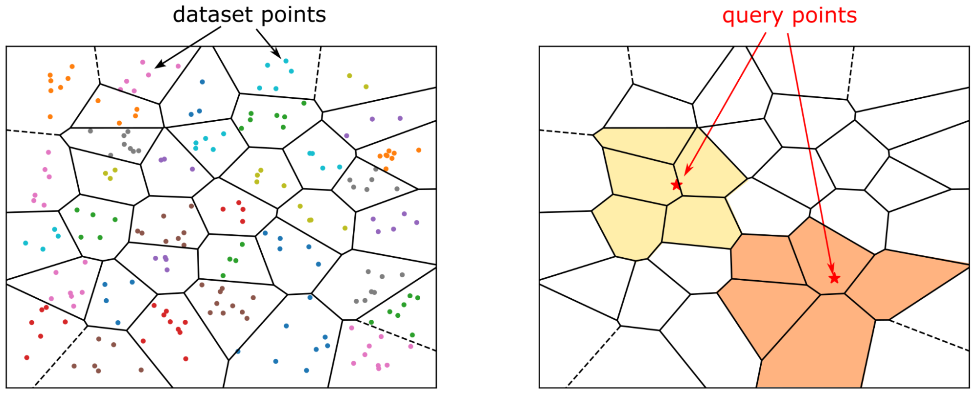
IVF works by partitioning a large dataset of vectors into smaller, manageable clusters, each represented by a central point called a "centroid." These centroids act as anchors for their respective partitions. During a search, the system quickly identifies the clusters whose centroids are closest to the query vector and only searches within those, ignoring the rest of the dataset.

IVF in Apache Doris

Apache Doris supports building IVF‑based ANN indexes starting from version 4.x.

Index Construction

The index type used here is ANN. There are two ways to create an ANN index: you can define it when creating the table, or you can use the CREATE/BUILD INDEX syntax. The two approaches differ in how and when the index is built, and therefore fit different scenarios.

Approach 1: define an ANN index on a vector column when creating the table. As data is loaded, an ANN index is built for each segment as it is created. The advantage is that once data loading completes, the index is already built and queries can immediately use it for acceleration. The downside is that synchronous index building slows down data ingestion and may cause extra index rebuilds during compaction, leading to some waste of resources.

CREATE TABLE sift_1M (
  id int NOT NULL,
  embedding array<float>  NOT NULL  COMMENT "",
  INDEX ann_index (embedding) USING ANN PROPERTIES(
      "index_type"="ivf",
      "metric_type"="l2_distance",
      "dim"="128",
      "nlist"="1024"
  )
) ENGINE=OLAP
DUPLICATE KEY(id) COMMENT "OLAP"
DISTRIBUTED BY HASH(id) BUCKETS 1
PROPERTIES (
  "replication_num" = "1"
);

INSERT INTO sift_1M
SELECT *
FROM S3(
  "uri" = "https://selectdb-customers-tools-bj.oss-cn-beijing.aliyuncs.com/sift_database.tsv",
  "format" = "csv");

CREATE/BUILD INDEX

Approach 2: CREATE/BUILD INDEX.

CREATE TABLE sift_1M (
  id int NOT NULL,
  embedding array<float>  NOT NULL  COMMENT ""
) ENGINE=OLAP
DUPLICATE KEY(id) COMMENT "OLAP"
DISTRIBUTED BY HASH(id) BUCKETS 1
PROPERTIES (
  "replication_num" = "1"
);

INSERT INTO sift_1M
SELECT *
FROM S3(
  "uri" = "https://selectdb-customers-tools-bj.oss-cn-beijing.aliyuncs.com/sift_database.tsv",
  "format" = "csv");

After data is loaded, you can run CREATE INDEX. At this point the index is defined on the table, but no index is yet built for the existing data.

CREATE INDEX idx_test_ann ON sift_1M (`embedding`) USING ANN PROPERTIES (
  "index_type"="ivf",
  "metric_type"="l2_distance",
  "dim"="128",
  "nlist"="1024"
);

SHOW DATA ALL FROM sift_1M;

mysql> SHOW DATA ALL FROM sift_1M;
+-----------+-----------+--------------+----------+----------------+---------------+----------------+-----------------+----------------+-----------------+
| TableName | IndexName | ReplicaCount | RowCount | LocalTotalSize | LocalDataSize | LocalIndexSize | RemoteTotalSize | RemoteDataSize | RemoteIndexSize |
+-----------+-----------+--------------+----------+----------------+---------------+----------------+-----------------+----------------+-----------------+
| sift_1M   | sift_1M   | 10           | 1000000  | 170.093 MB     | 170.093 MB    | 0.000          | 0.000           | 0.000          | 0.000           |
|           | Total     | 10           |          | 170.093 MB     | 170.093 MB    | 0.000          | 0.000           | 0.000          | 0.000           |
+-----------+-----------+--------------+----------+----------------+---------------+----------------+-----------------+----------------+-----------------+

Then you can build the index using the BUILD INDEX statement:

BUILD INDEX idx_test_ann ON sift_1M;

BUILD INDEX is executed asynchronously. You can use SHOW BUILD INDEX (in some versions SHOW ALTER) to check the job status.

SHOW BUILD INDEX WHERE TableName = "sift_1M";

mysql> SHOW BUILD INDEX WHERE TableName = "sift_1M";
+---------------+-----------+---------------+-----------------------------------------------------------------------------------------------------------------------------------------------------+-------------------------+-------------------------+---------------+----------+------+----------+
| JobId         | TableName | PartitionName | AlterInvertedIndexes                                                                                                                                | CreateTime              | FinishTime              | TransactionId | State    | Msg  | Progress |
+---------------+-----------+---------------+-----------------------------------------------------------------------------------------------------------------------------------------------------+-------------------------+-------------------------+---------------+----------+------+----------+
| 1764392359610 | sift_1M   | sift_1M       | [ADD INDEX idx_test_ann (`embedding`) USING ANN PROPERTIES("dim" = "128", "index_type" = "ivf", "metric_type" = "l2_distance", "nlist" = "1024")],  | 2025-12-01 14:18:22.360 | 2025-12-01 14:18:27.885 | 5036          | FINISHED |      | NULL     |
+---------------+-----------+---------------+-----------------------------------------------------------------------------------------------------------------------------------------------------+-------------------------+-------------------------+---------------+----------+------+----------+
1 row in set (0.00 sec)

mysql> SHOW DATA ALL FROM sift_1M;
+-----------+-----------+--------------+----------+----------------+---------------+----------------+-----------------+----------------+-----------------+
| TableName | IndexName | ReplicaCount | RowCount | LocalTotalSize | LocalDataSize | LocalIndexSize | RemoteTotalSize | RemoteDataSize | RemoteIndexSize |
+-----------+-----------+--------------+----------+----------------+---------------+----------------+-----------------+----------------+-----------------+
| sift_1M   | sift_1M   | 10           | 1000000  | 671.084 MB     | 170.093 MB    | 500.991 MB     | 0.000           | 0.000          | 0.000           |
|           | Total     | 10           |          | 671.084 MB     | 170.093 MB    | 500.991 MB     | 0.000           | 0.000          | 0.000           |
+-----------+-----------+--------------+----------+----------------+---------------+----------------+-----------------+----------------+-----------------+
2 rows in set (0.00 sec)

DROP INDEX

You can drop an unsuitable ANN index with ALTER TABLE sift_1M DROP INDEX idx_test_ann. Dropping and recreating indexes is common during hyperparameter tuning, when you need to test different parameter combinations to achieve the desired recall.

Querying

ANN indexes support both Top‑N search and range search.

When the vector column has high dimensionality, the literal representation of the query vector itself can incur extra parsing overhead. Therefore, directly embedding the full query vector into raw SQL is not recommended in production, especially under high concurrency. A better practice is to use prepared statements, which avoid repetitive SQL parsing.

We recommend using the doris-vector-search python library, which wraps the necessary operations for vector search in Doris based on prepared statements, and includes data conversion utilities that map Doris query results into Pandas DataFrames for convenient downstream AI application development.

from doris_vector_search import DorisVectorClient, AuthOptions

auth = AuthOptions(
    host="127.0.0.1",
    query_port=9030,
    user="root",
    password="",
)

client = DorisVectorClient(database="test", auth_options=auth)

tbl = client.open_table("sift_1M")

query = [0.1] * 128  # Example 128-dimensional vector

# SELECT id FROM sift_1M ORDER BY l2_distance_approximate(embedding, query) LIMIT 10;
result = tbl.search(query, metric_type="l2_distance").limit(10).select(["id"]).to_pandas()

print(result)

Sample output:

       id
0  123911
1  926855
2  123739
3   73311
4  124493
5  153178
6  126138
7  123740
8  125741
9  124048

Recall Optimization

In vector search, recall is the most important metric; performance numbers only make sense under a given recall level. The main factors that affect recall are:

1. Index‑time parameter of IVF (nlist) and query-time parameter (nprobe).
2. Vector quantization.
3. Segment size and the number of segments.

This article focuses on the impact of (1) and (3) on recall. Vector quantization will be covered in a separate document.

Index Hyperparameters

An IVF index organizes vectors into multiple clusters. During index construction, vectors are partitioned into groups using clustering. The search process then focuses only on the most relevant clusters. The workflow is roughly as follows:

At index time:

1. Clustering: All vectors are partitioned into nlist clusters using a clustering algorithm (e.g., k‑means). The centroid of each cluster is computed and stored.
2. Vector assignment: Each vector is assigned to the cluster whose centroid is closest to it, and the vector is added to that cluster’s inverted list.

At query time:

1. Cluster selection using nprobe: For a query vector, distances to all nlist centroids are computed. Only the nprobe closest clusters are selected for searching.
2. Exhaustive search within selected clusters: The query is compared against every vector in the selected nprobe clusters to find the nearest neighbors.

In summary:

nlist defines the number of clusters (inverted lists). It affects recall, memory overhead, and build time. A larger nlist creates finer‑grained clusters, which can improve search speed if the query’s nearest neighbors are well‑localized, but it also increases the cost of clustering and the risk of neighbors being spread across multiple clusters.

nprobe defines the number of clusters to search during a query. A larger nprobe increases recall and query latency (more vectors are examined). A smaller nprobe makes queries faster but may miss neighbors that reside in non‑probed clusters.

By default, Doris uses nlist = 1024 and nprobe = 64.

The above is a qualitative analysis of these two hyperparameters. The following table shows empirical results on the SIFT_1M dataset:

nlist	nprobe	recall_at_100
1024	64	0.9542
1024	32	0.9034
1024	16	0.8299
1024	8	0.7337
512	32	0.9384
512	16	0.8763
512	8	0.7869

It is hard to provide one single optimal setting in advance, but you can follow a practical workflow for hyperparameter selection:

1. Create a table table_multi_index without indexes. It can contain 2 or 3 vector columns.
2. Load data into table_multi_index using Stream Load or other ingestion methods.
3. Use CREATE INDEX and BUILD INDEX to build ANN indexes on all vector columns.
4. Use different index parameter configurations on different columns. After index building finishes, compute recall on each column and choose the best parameter combination.

for exmaple:

ALTER TABLE tbl DROP INDEX idx_embedding;
CREATE INDEX idx_embedding ON tbl (`embedding`) USING ANN PROPERTIES (
  "index_type"="ivf",
  "metric_type"="inner_product",
  "dim"="768",
  "nlist"="1024"
);
BUILD INDEX idx_embedding ON tbl;

Number of Rows Covered per Index

Internally, Doris organizes data in multiple layers.

• At the top is a table, which is partitioned into N tablets using a distribution key. Tablets serve as units for data sharding, relocation, and rebalance.
• Each data ingestion or compaction produces a new rowset under a tablet. A rowset is a versioned collection of data.
• Data in a rowset is actually stored in segment files.

Similar to inverted indexes, vector indexes are built at the segment level. The segment size is determined by BE configuration options like write_buffer_size and vertical_compaction_max_segment_size. During ingestion and compaction, when the in‑memory memtable reaches a certain size, it is flushed to disk as a segment file, and a vector index (or multiple indexes for multiple vector columns) is built for that segment. The index only covers the rows in that segment.

Given a fixed set of IVF parameters, there is always a limit to the number of vectors for which the index can still maintain high recall. Once the number of vectors in a segment grows beyond that limit, recall starts to degrade.

You can use SHOW TABLETS FROM table to inspect the compaction status of a table. By following the corresponding URL, you can see how many segments it has.

Impact of Compaction on Recall

Compaction can affect recall because it may create larger segments, which can exceed the “coverage capacity” implied by the original hyperparameters. As a result, the recall level achieved before compaction may no longer hold after compaction.

We recommend triggering a full compaction before running BUILD INDEX. Building indexes on fully compacted segments stabilizes recall and also reduces write amplification caused by index rebuilds.

Query Performance

Cold Loading of Index Files

The IVF ANN index in Doris is implemented using Meta’s open‑source library Faiss. IVF indexes become effective after being loaded into memory. Therefore, before running high‑concurrency workloads, it is recommended to run some warm‑up queries to make sure that all relevant segment indexes are loaded into memory; otherwise, disk I/O overhead can significantly hurt query performance.

Memory Footprint vs. Performance

Without quantization or compression, the memory footprint of an IVF index is roughly 1.02-1.1× the memory footprint of all vectors it indexes.

For example, with 1 million 128‑dimensional vectors, an IVF-FLAT index requires approximately:

128 * 4 * 1,000,000 * 1.02 ≈ 500 MB.

Some reference values:

dim	rows	estimated memory
128	1M	496 MB
768	1M	2.9 GB

To maintain stable performance, ensure that each BE has enough memory; otherwise, frequent swapping and I/O on index files will severely degrade query latency.

Benchmark

When benchmark, the deployment model should follow the production environment setup, with FE and BE deployed separately, and the client should run on another independent machine.

You can use VectorDBBench as benchmark framekwork.

Performance768D1M

Benchmark command:

# load
NUM_PER_BATCH=1000000 python3 -m vectordbbench doris --host 127.0.0.1 --port 9030 --case-type Performance768D1M --db-name Performance768D1M --stream-load-rows-per-batch 500000 --index-prop index_type=ivf,nlist=1024 --skip-search-serial --skip-search-concurrent

# search
NUM_PER_BATCH=1000000 python3 -m vectordbbench doris --host 127.0.0.1 --port 9030 --case-type Performance768D1M --db-name Performance768D1M --search-concurrent --search-serial --num-concurrency 10,40,80 --stream-load-rows-per-batch 500000 --index-prop index_type=ivf,nlist=1024 --session-var ivf_nprobe=64 --skip-load --skip-drop-old