Apache Doris Overview
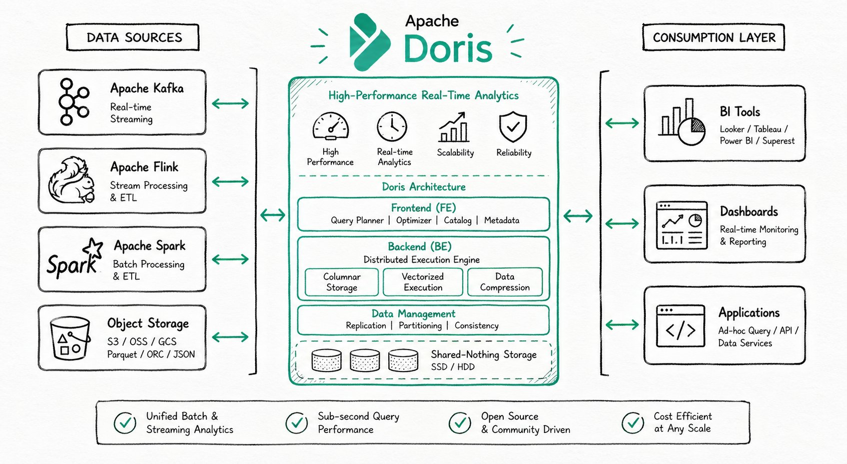
Apache Doris is a high-performance, real-time analytical database based on the MPP architecture. Known for being efficient, simple, and unified, it returns query results over massive datasets within sub-second latency, and a single system supports both high-concurrency point queries and high-throughput complex analytics.
Core Highlights
| Capability | Data |
|---|---|
| Query latency | < 1 second (sub-second response) |
| Ingestion latency | Second-level (real-time data ingestion) |
| Concurrency | 10,000+ QPS |
| Storage scale | PB-level / hundreds of machines per cluster |
| SQL interface | MySQL protocol-compatible layer, ANSI SQL syntax |
Typical Use Cases
Apache Doris is widely used in the following three categories of scenarios:
Real-Time Data Analytics
Internal and external real-time reports, dashboards, user behavior analysis, A/B testing platforms, and log search and analysis.
Representative cases:
- Real-time dashboards: Singles' Day order volume monitoring with second-level updates
- User profile analysis: audience segmentation and precision marketing
- Log search and analysis: troubleshooting and performance optimization
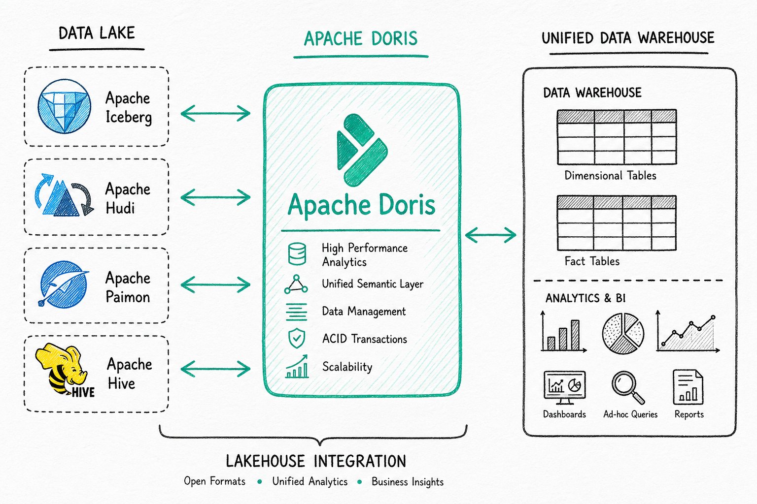
Lakehouse Analytics
Unified data warehouse construction, federated query acceleration over data lakes, and mixed workload analytics.
Hybrid Search and Analytics (AI Data Stack)
In the era of large models, Apache Doris deeply integrates full-text search, vector search, and AI function capabilities, building a complete AI data stack that spans data storage, retrieval, and analytics.
| Scenario | Description |
|---|---|
| Agent Facing Analytics | Millisecond-level real-time decision making for AI agents (fraud detection, intelligent recommendations) |
| Hybrid search and analytics | Run vector similarity search, keyword filtering, and aggregate analytics together in a single SQL statement |
| RAG applications | Enterprise knowledge base Q&A, intelligent customer service, and document assistants |
| Semantic search | Cross-language retrieval, synonym recognition, and intent understanding |
| AI observability | Model training monitoring, inference tracing, and log analysis |
System Architecture
Apache Doris is highly compatible with the MySQL protocol, supports standard SQL, can be accessed by various client tools, and integrates seamlessly with BI tools. When deploying Apache Doris, you can choose either the integrated storage and compute architecture or the decoupled storage and compute architecture based on business needs.
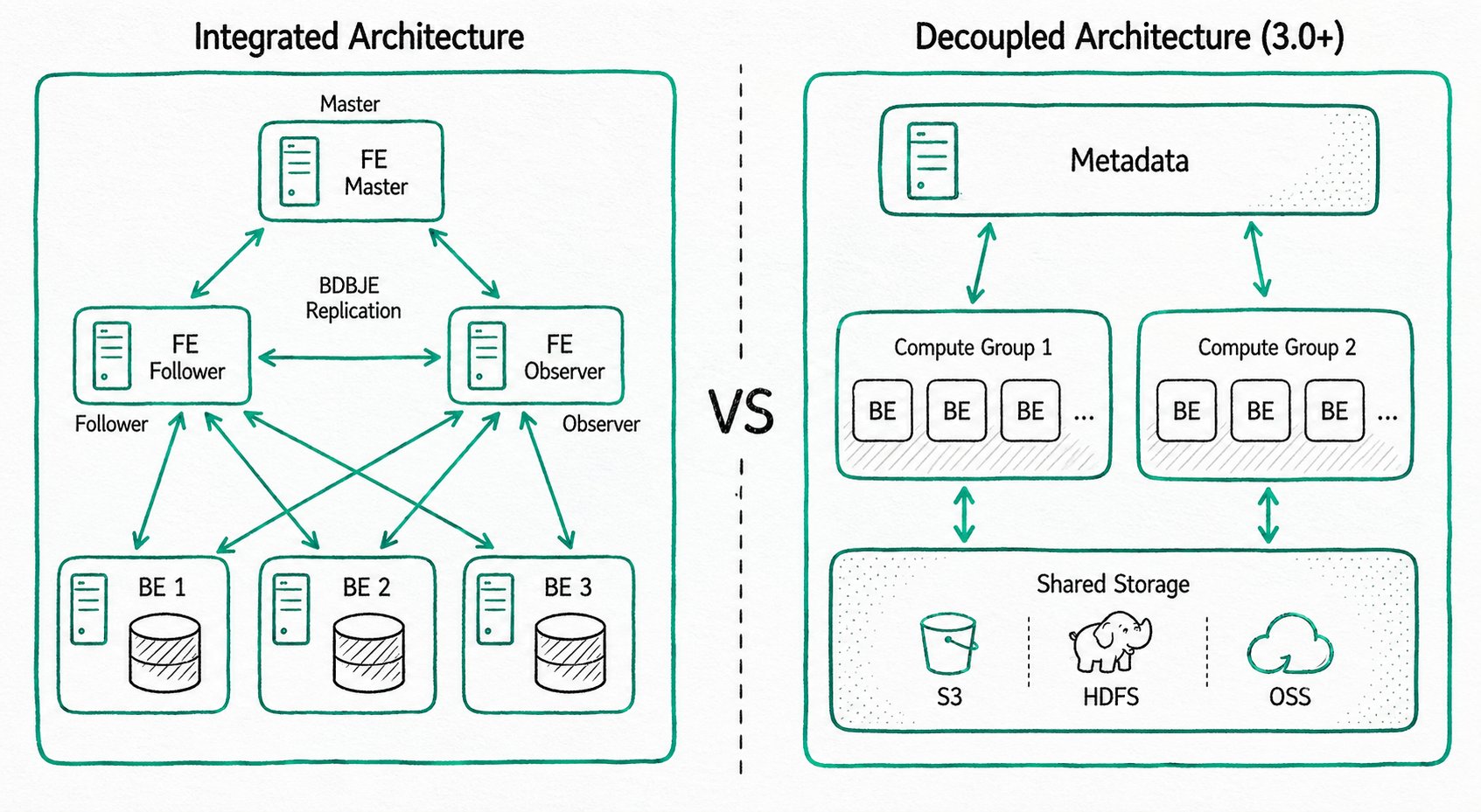
Integrated Storage and Compute Architecture
A streamlined architecture that contains two types of processes:
- Frontend (FE): receives requests, parses queries, manages metadata, and manages nodes
- Backend (BE): stores data and executes queries (with multi-replica storage)
In production, multiple FE nodes are deployed for high availability. FE nodes have three roles: Master, Follower, and Observer.
Decoupled Storage and Compute Architecture (Shared Storage)
Storage and compute are separated, so you can scale storage capacity and compute resources independently:
- Compute layer: multiple compute groups, each of which can serve as an independent tenant
- Storage layer: shared storage such as S3, HDFS, or OSS
How to choose: if your business scale is manageable and you prefer simple operations, choose the integrated architecture. If you need elastic scaling, choose the decoupled architecture.
Technical Features
Storage Engine
Apache Doris uses columnar storage technology, encoding, compressing, and reading data column by column. This achieves an extremely high compression ratio while reducing scans of irrelevant data, making more effective use of IO and CPU resources. Doris is deeply optimized for ultra-wide table scenarios (10,000+ columns), ensuring efficient storage and queries for sparse columns. To meet the needs of different business scenarios, Doris provides multiple index structures (Sorted Compound Key, Min/Max, BloomFilter, inverted index, vector index) and storage models (Duplicate model, Aggregate model, Unique model), and supports strongly consistent single-table materialized views and asynchronously refreshed multi-table materialized views.
- Columnar storage: column-wise encoding, compression, and reading; high compression ratio plus reduced IO
- Multiple indexes: Sorted Compound Key, Min/Max, BloomFilter, inverted index, vector index
- Storage models: Duplicate model, Aggregate model, Unique model (supports row-level updates)
- Materialized views: strongly consistent single-table materialized views plus asynchronous multi-table materialized views
Vector indexes and inverted indexes are the core technologies that support Hybrid Search (hybrid search and analytics). For details, see AI Overview.
Query Engine
The Apache Doris query engine is based on the MPP (Massively Parallel Processing) architecture and supports both inter-node and intra-node parallel execution, as well as distributed Shuffle Join across multiple large tables. In complex multi-table join scenarios, Doris uses global query planning, distributed join strategies, and Runtime Filter technology to greatly reduce data transfer and accelerate join performance. Doris uses vectorized execution: all in-memory structures use a columnar layout, which significantly reduces virtual function calls, improves cache hit rates, and effectively uses SIMD instructions, delivering a 5-10x performance improvement in wide-table aggregation scenarios. Combined with Adaptive Query Execution (AQE) and the Pipeline execution engine, Doris dynamically optimizes execution plans based on runtime statistics and fully utilizes multi-core CPU capabilities.
- MPP architecture: inter-node and intra-node parallel execution, distributed Shuffle Join for large tables
- Vectorized execution: columnar in-memory layout, SIMD instructions, 5-10x performance improvement
- Adaptive Query Execution (AQE): Runtime Filter dynamically optimizes joins
- Pipeline execution engine: parallelism across multi-core CPUs, with thread-count limits to address thread bloat
Hybrid Search Capabilities (AI Enhanced)
Apache Doris combines structured analytics, full-text search, and vector search in a single SQL statement. A single system supports vector similarity search, keyword filtering, and aggregate analytics together, with no data migration or heterogeneous system integration required. Combined with the VARIANT type, which natively supports dynamic JSON structures, and Light Schema Change, which lets you change fields in seconds, Doris provides efficient data support for AI scenarios such as RAG applications, semantic search, and enterprise knowledge bases.
SELECT * FROM products
WHERE match(query_vector, 'summer breathable shoes')  -- Vector similarity search
  AND body MATCH 'breathable lightweight'           -- Full-text keyword search
  AND category_id = 1                                -- Structured filtering
GROUP BY brand
ORDER BY sales_count DESC;
- Unified architecture: no data migration, no heterogeneous systems
- Hybrid query performance: a single SQL statement runs vector, keyword, and aggregate operations together
- VARIANT type: native support for dynamic JSON, with Light Schema Change for second-level field changes
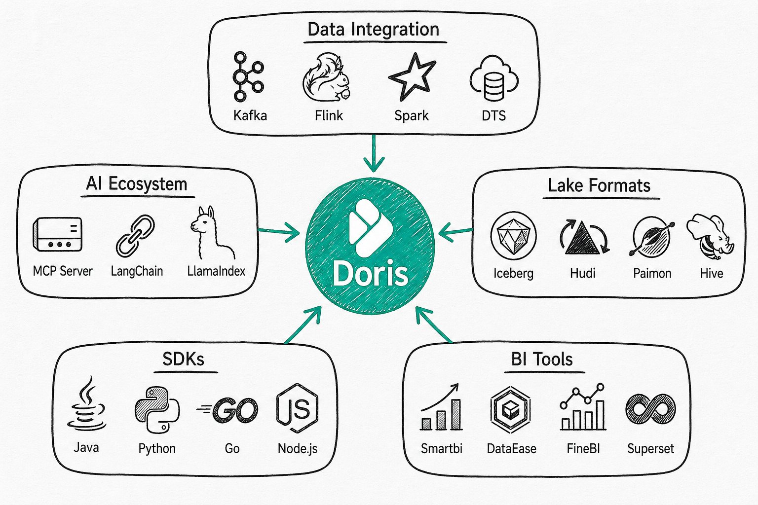
Ecosystem Integration
Apache Doris integrates deeply with mainstream data ecosystems.
Community and Contribution
You are welcome to join the community: https://doris.apache.org/community/join-community