Data Bucketing

A partition can further be divided into different data buckets based on business logic. Each bucket will be stored as a physical data tablet. A reasonable bucket strategy can effectively reduce the amount of data scanned during queries, thereby improving query performance and increasing query concurrency.

Bucket Methods

Doris supports two bucket methods: Hash Bucketing and Random Bucketing.

Hash Bucketing

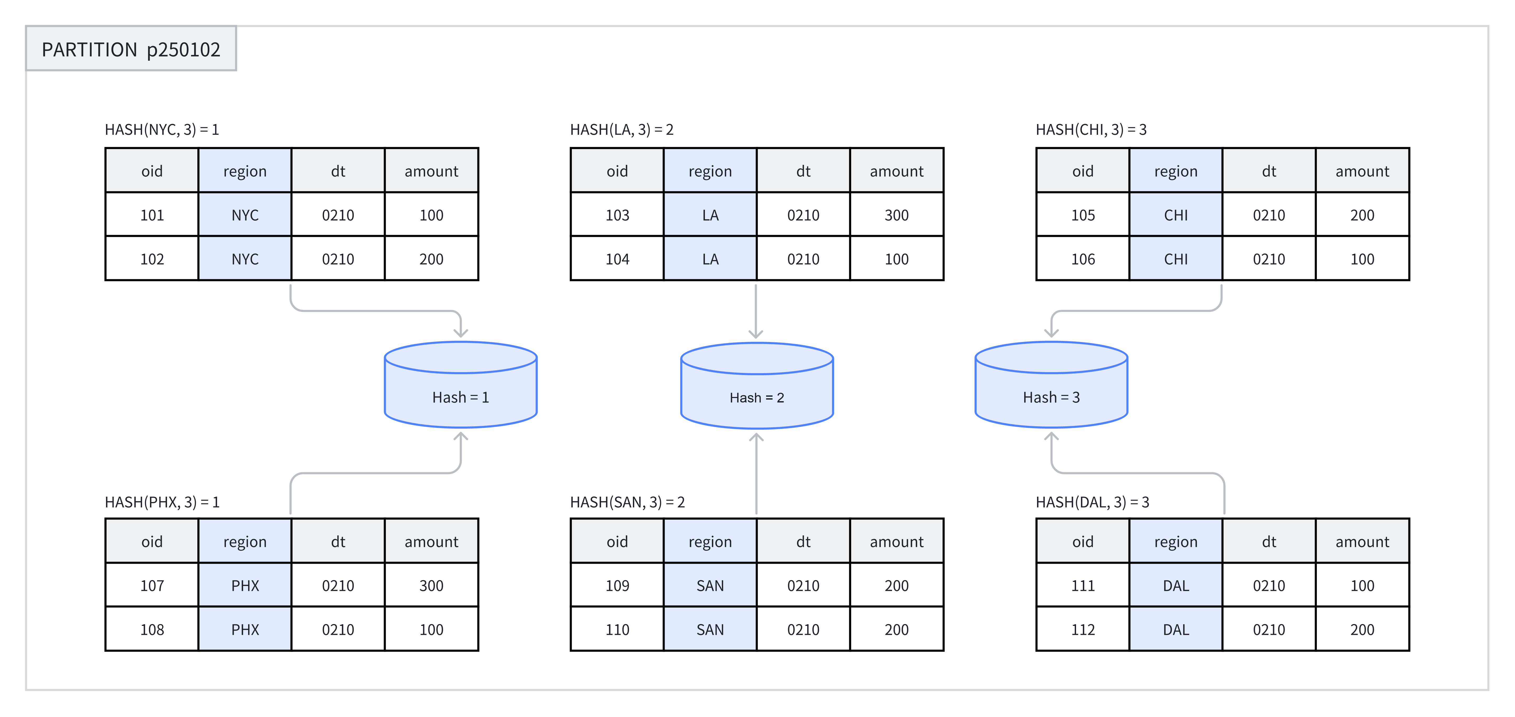
When creating a table or adding a partition, users need to select one or more columns as the bucket columns and specify the number of buckets. Within the same partition, the system performs a hash calculation based on the bucket key and the number of buckets. Data with the same hash value will be allocated to the same bucket. For example, in the figure below, partition p250102 is divided into three buckets based on the region column, and rows with the same hash value are placed into the same bucket.

It is recommended to use Hash Bucketing in the following scenarios:

• When the business needs to frequently filter based on a certain field, you can use this field as the bucket key for Hash Bucketing to improve query efficiency.

• When the data distribution in the table is relatively uniform, Hash Bucketing is also a suitable choice.

The following example shows how to create a table with Hash Bucketing. For detailed syntax, please refer to the CREATE TABLE statement.

CREATE TABLE demo.hash_bucket_tbl(
    oid         BIGINT,
    dt          DATE,
    region      VARCHAR(10),
    amount      INT
)
DUPLICATE KEY(oid)
PARTITION BY RANGE(dt) (
    PARTITION p250101 VALUES LESS THAN("2025-01-01"),
    PARTITION p250102 VALUES LESS THAN("2025-01-02")
)
DISTRIBUTED BY HASH(region) BUCKETS 8;

In the example, DISTRIBUTED BY HASH(region) specifies the creation of Hash Bucketing and selects the region column as the bucket key. Meanwhile, BUCKETS 8 specifies the creation of 8 buckets.

Random Bucketing

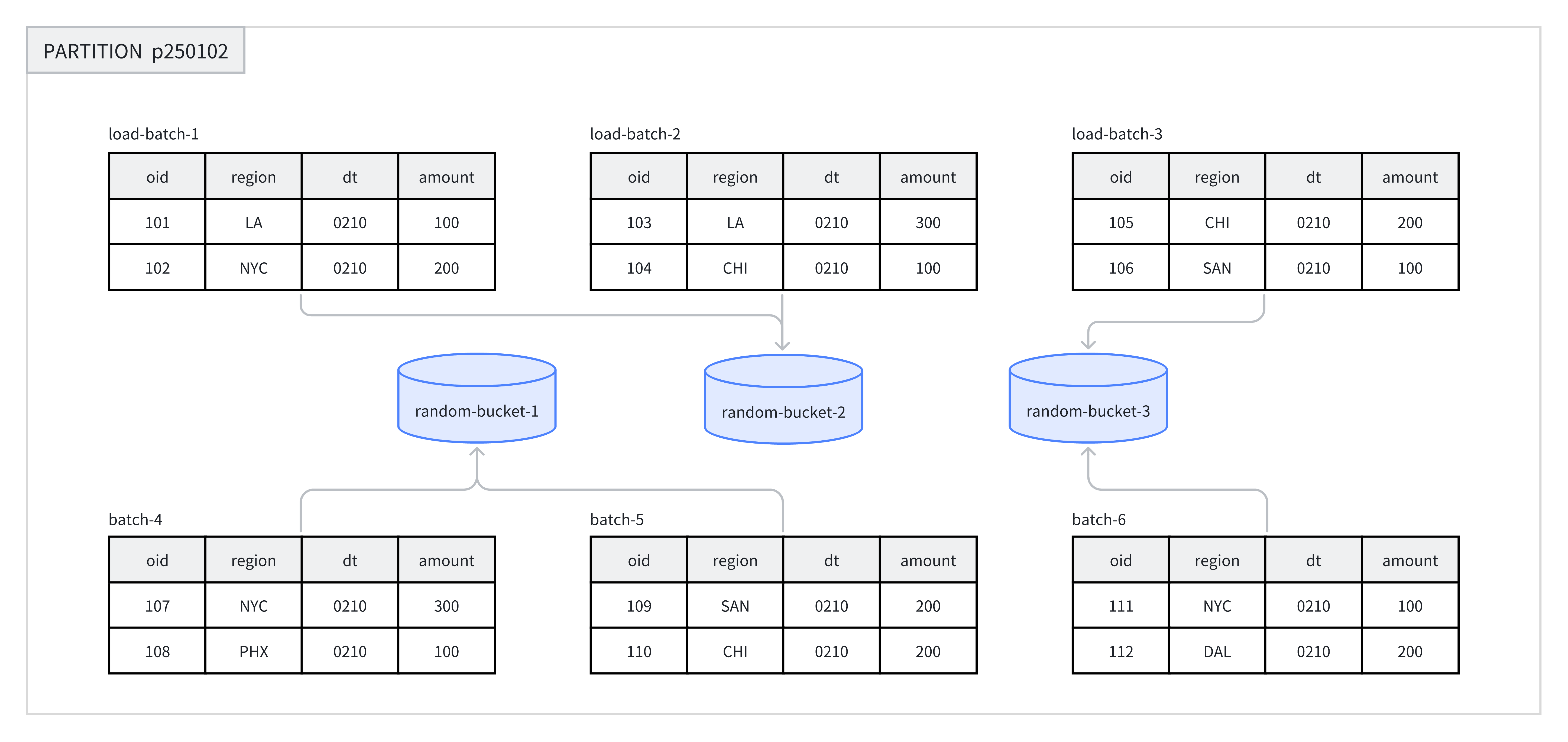
In each partition, Random Bucketing randomly distributes data to various buckets without relying on the hash value of a certain field. Random Bucketing ensures uniform data distribution, thus avoiding data skew caused by improper bucket key selection.

During data import, each batch of a single import job will be randomly written to a tablet, ensuring uniform data distribution. For example, in one operation, eight batches of data are randomly allocated to three buckets under partition p250102.

When using Random Bucketing, you can enable the single-tablet import mode (set load_to_single_tablet to true). During large-scale data imports, one batch of data will only be written to one data tablet, helping to improve the concurrency and throughput of data imports, reducing write amplification caused by data imports and Compaction, thereby ensuring cluster stability.

It is recommended to use Random Bucketing in the following scenarios:

• In scenarios of arbitrary dimension analysis, where the business does not frequently filter or join queries based on a specific column, you can choose Random Bucketing.

• When the data distribution of frequently queried columns or combinations of columns is extremely uneven, using Random Bucketing can avoid data skew.

• Random Bucketing cannot be pruned based on bucket keys and will scan all data in the hit partition, so it is not recommended for point query scenarios.

• Only DUPLICATE tables can use Random partitioning. UNIQUE and AGGREGATE tables cannot use Random Bucketing.

The following example shows how to create a table with Random Bucketing. For detailed syntax, please refer to the CREATE TABLE statement:

CREATE TABLE demo.random_bucket_tbl(
    oid         BIGINT,
    dt          DATE,
    region      VARCHAR(10),
    amount      INT
)
DUPLICATE KEY(oid)
PARTITION BY RANGE(dt) (
    PARTITION p250101 VALUES LESS THAN("2025-01-01"),
    PARTITION p250102 VALUES LESS THAN("2025-01-02")
)
DISTRIBUTED BY RANDOM BUCKETS 8;

In the example, the statement DISTRIBUTED BY RANDOM specifies the use of Random Bucketing. Creating Random Bucketing does not require selecting a bucket key, and the statement BUCKETS 8 specifies the creation of 8 buckets.

Choosing Bucket Keys

Note

Only Hash Bucketing requires selecting bucket keys; Random Bucketing does not require selecting bucket keys.

Bucket keys can be one or more columns. If it is a DUPLICATE table, any Key column or Value column can be used as the bucket key. If it is an AGGREGATE or UNIQUE table, to ensure gradual aggregation, the bucket column must be a Key column.

Generally, you can choose bucket keys based on the following rules:

• Using Query Filter Conditions: Using query filter conditions for Hash Bucketing helps data pruning and reduces data scan volume;

• Using High Cardinality Columns: Selecting high cardinality (many unique values) columns for Hash Bucketing helps to evenly distribute data across each bucket;

• High-Concurrency Point Query Scenarios: It is recommended to select a single column or fewer columns for bucketing. Point queries may only trigger a scan of one bucket, and the probability of different queries triggering scans of different buckets is high, thereby reducing the IO impact between queries.

• High-Throughput Query Scenarios: It is recommended to select multiple columns for bucketing to make data more evenly distributed. If the query conditions cannot include the equality conditions of all bucket keys, it will increase query throughput and reduce the latency of single queries.

Choosing the Number of Buckets

In Doris, a bucket is stored as a physical file (tablet). The number of tablets in a table equals partition_num (number of partitions) multiplied by bucket_num (number of buckets). Once the number of Partitions is specified, it cannot be changed.

When determining the number of buckets, you need to consider machine expansion in advance. Starting from version 2.0, Doris supports automatically setting the number of buckets in partitions based on machine resources and cluster information.

Manually Setting the Number of Buckets

You can specify the number of buckets using the DISTRIBUTED statement:

-- Set hash bucket num to 8
DISTRIBUTED BY HASH(region) BUCKETS 8

-- Set random bucket num to 8
DISTRIBUTED BY RANDOM BUCKETS 8

When determining the number of buckets, two principles are usually followed: quantity and size. If there is a conflict between the two, the size principle is prioritized:

• Size Principle: It is recommended that the size of a tablet should be within the range of 1-10GB. Too small a tablet may result in poor aggregation effect and increase metadata management pressure; too large a tablet is not conducive to replica migration and supplementation and will increase the cost of retrying Schema Change operations.

• Quantity Principle: Without considering expansion, it is recommended that the number of tablets for a table be slightly more than the number of disks in the entire cluster.

For example, assuming there are 10 BE machines with one disk per BE, you can follow the recommendations below for data bucketing:

Table Size	Recommended Number of Buckets
500MB	4-8 buckets
5GB	6-16 buckets
50GB	32 buckets
500GB	Partition recommended, 50GB per partition, 16-32 buckets per partition
5TB	Partition recommended, 50GB per partition, 16-32 buckets per partition

Note

The data volume of the table can be viewed using the SHOW DATA command. The result needs to be divided by the number of replicas and the data volume of the table.

Automatic Bucket Number Setting

The automatic bucket number calculation function will automatically predict the future partition size based on the partition size over a period of time, and determine the number of buckets accordingly.

-- Set hash bucket auto
DISTRIBUTED BY HASH(region) BUCKETS AUTO
properties("estimate_partition_size" = "20G")

-- Set random bucket auto
DISTRIBUTED BY HASH(region) BUCKETS AUTO
properties("estimate_partition_size" = "20G")

When creating buckets, you can adjust the estimated partition size through the estimate_partition_size attribute. This parameter is optional, and if not provided, Doris will default to 10GB. Please note that this parameter is not related to the future partition size calculated by the system based on historical partition data.

Maintaining Data Buckets

Note

Currently, Doris only supports modifying the number of buckets in newly added partitions and does not support the following operations:

1. Modifying the bucketing type
2. Modifying the bucket key
3. Modifying the number of buckets for existing buckets

When creating a table, the number of buckets for each partition is uniformly specified through the DISTRIBUTED statement. To cope with data growth or reduction, you can specify the number of buckets for the new partition when dynamically adding partitions. The following example shows how to modify the number of buckets in newly added partitions using the ALTER TABLE command:

-- Modify hash bucket table
ALTER TABLE demo.hash_bucket_tbl 
ADD PARTITION p250103 VALUES LESS THAN("2025-01-03")
DISTRIBUTED BY HASH(region) BUCKETS 16;

-- Modify random bucket table
ALTER TABLE demo.random_bucket_tbl 
ADD PARTITION p250103 VALUES LESS THAN("2025-01-03")
DISTRIBUTED BY RANDOM BUCKETS 16;

-- Modify dynamic partition table
ALTER TABLE demo.dynamic_partition_tbl
SET ("dynamic_partition.buckets"="16");

After modifying the number of buckets, you can use the SHOW PARTITION command to check the updated number of buckets.