Doris analysis: Doris SQL principle analysis
Lead: This article mainly introduces the principle of Doris SQL parsing.
It focuses on generating a single-machine logical plan, developing a distributed logical plan, and generating a distributed physical plan. Analyze, SinglePlan, DistributedPlan, and Schedule four parts correspond to the code implementation.
First, AST will be processed preliminary by Analyze and then optimized by SinglePlan to generate a single-machine query plan. Third, DistributedPlan will split the single-machine query plan into distributed query plans. In the end, the query plan will be sent to machines and executed orderly, which decide by Schedule.
Since there are many types of SQL, this article focuses on the analysis of query SQL. Doris's SQL analysis will be explained deeply in the algorithm principle and code implementation.
Doris is an interactive SQL database based on MPP architecture, mainly used to solve near real-time reports and multi-dimensional analysis. The Doris architecture is straightforward, with only two types of processes.
-
Frontend(FE): It is mainly responsible for user request access, query parsing and planning, storage and management of metadata, and node management-related work.
-
Backend(BE): It is mainly responsible for data storage and query plan execution.
In Doris' storage engine, data will be horizontally divided into several data shards (Tablet, also called data bucket). Each tablet contains several rows of data. Multiple Tablets belong to different partitions logically. A Tablet only belongs to one Partition. And a Partition contains several Tablets. Tablet is the smallest physical storage unit for operations such as data movement, copying, etc.
2. SQL parsing In Apache Doris
SQL parsing in this article refers to the process of generating a complete physical execution plan after a series of parsing of an SQL statement.
This process includes the following four steps: lexical analysis, syntax analysis, generating a logical plan, and generating a physical plan.
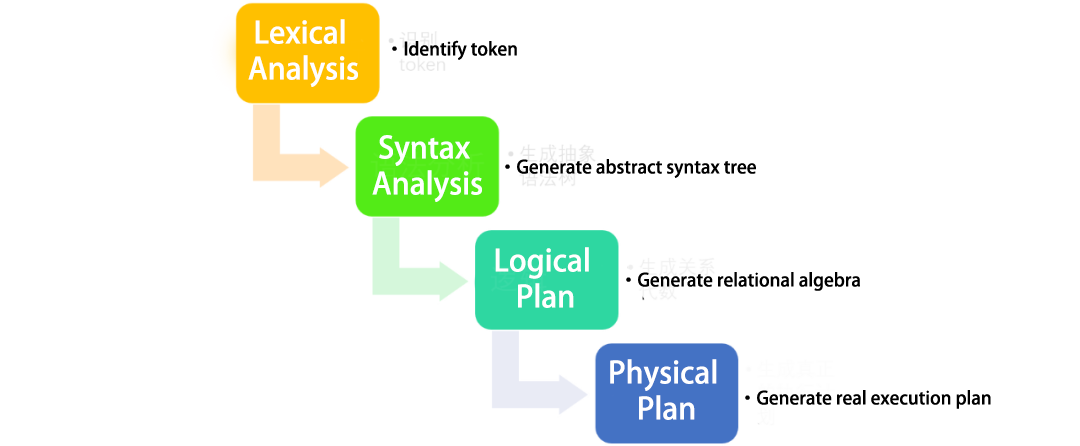
2.1 Lexical analysis
The lexical analysis will identify the SQL in the form of a string into tokens, in preparation for the grammatical analysis.
select ......  from ...... where ....... group by ..... order by ......

SQL Tokens could be divided into the following categories:
○ Keywords (select, from, where)
○ operator (+, -, >=)
○ Open/close flag ((, CASE)
○ placeholder (?)
○ Comments
○ space
......
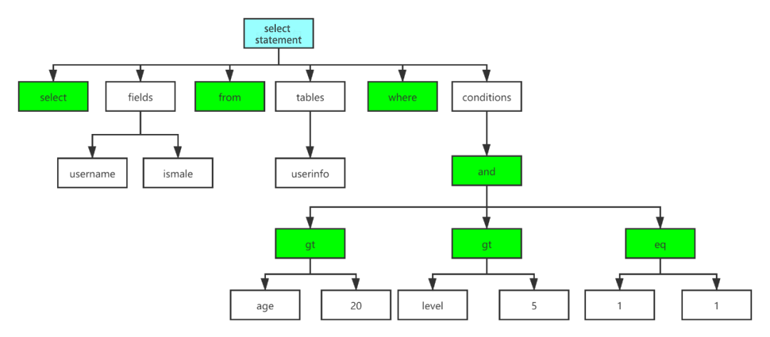
2.2 Syntax analysis
The syntax analysis will convert the token generated by the lexical analysis into an abstract syntax tree based on the syntax rules, as shown in Figure 2.
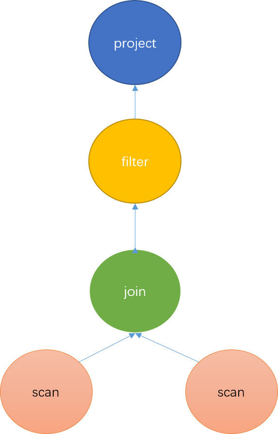
2.3 Logical plan
The logical plan converts the abstract syntax tree into an algebraic relation, which is an operator tree, and each node represents a calculation method for data. The entire tree represents the calculation method and flows direction of data, as shown in Figure 3.
2.4 Physical plan
The physical plan is the plan that determines which computing operations are performed on which machines. It will be generated based on the logical plan, the distribution of machines, and the distribution of data.
The SQL parsing of the Doris system also adopts these steps, but it is refined and optimized according to the characteristics of the Doris system structure and the storage method of data to maximize the computing power of the machine.
3. Design goals
The design goals of the Doris SQL parsing architecture are:
-
Maximize Computational Parallelism
-
Minimize network transfer of data
-
Minimize the amount of data that needs to be scanned
4. Architecture
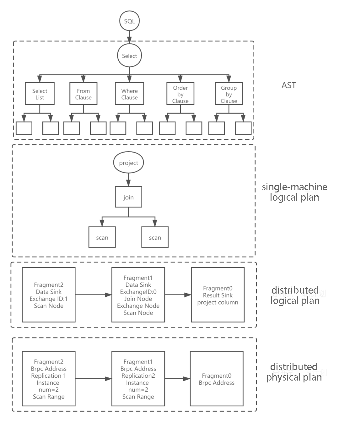
Doris SQL parsing includes five steps: lexical analysis, syntax analysis, generation of a stand-alone logical plan, generation of a distributed logical plan, and generation of a physical execution plan.
In terms of code implementation, it corresponds to the following five steps: Parse, Analyze, SinglePlan, DistributedPlan, and Schedule, which as shown in Figure 4.
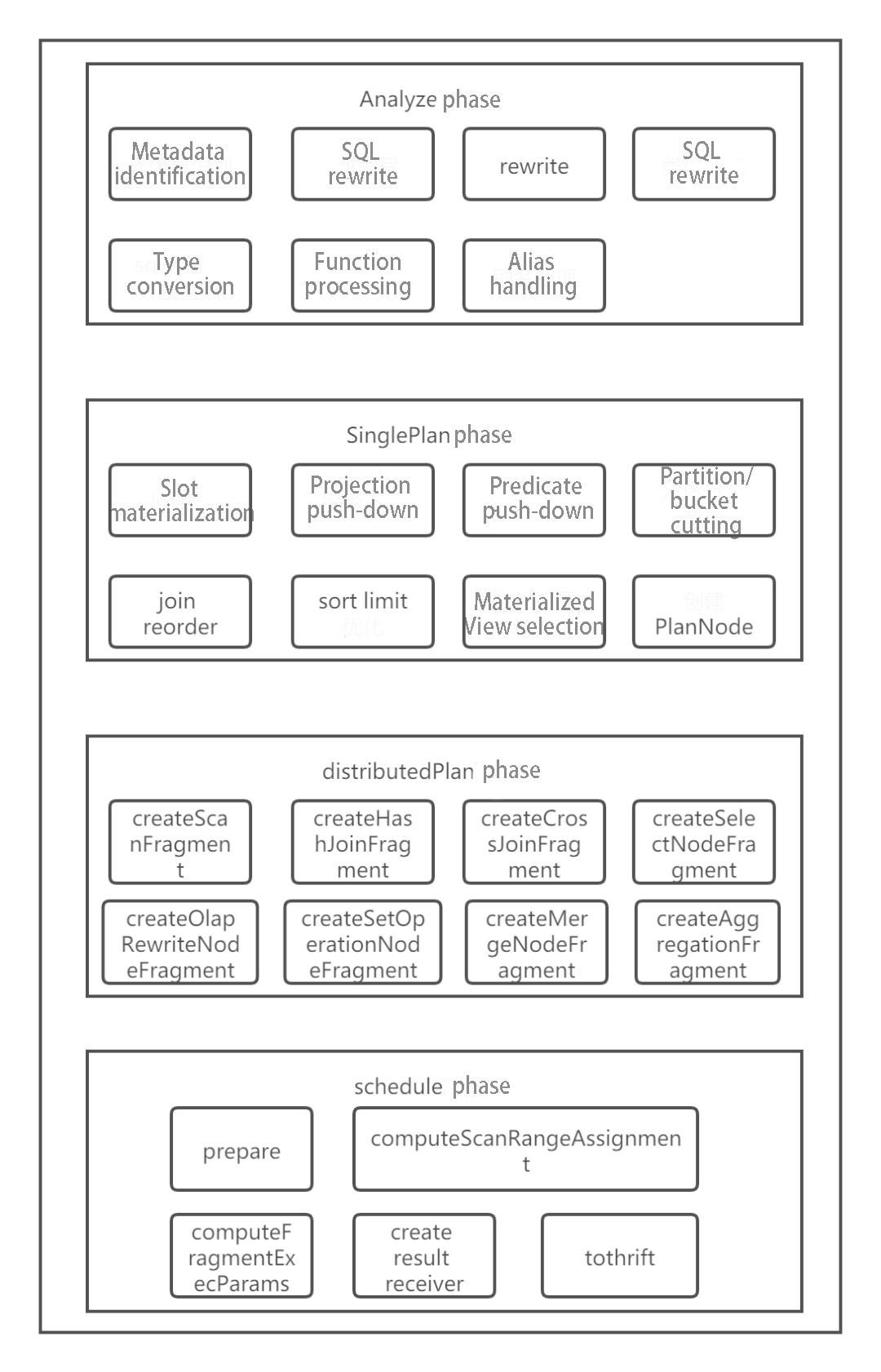
The Parse phase will not be discussed in this article. Analyze will do some pre-processing of the AST. A stand-alone query plan will be optimized by SinglePlan based on the AST. DistributedPlan will split the stand-alone query plan into distributed query plans. Schedule phase will determine which machines the query plan will be sent to for execution.
Since there are many types of SQL, this article focuses on the analysis of query SQL.
Figure 5 shows a simple query SQL parsing implementation in Doris.
5. Parse Phase
In the Parse stage, JFlex technology is used for lexical analysis, java cup parser technology is used for syntax analysis, and an AST(Abstract Syntax Tree)will finally generate. These are existing and mature technologies and will not be introduced in detail here.
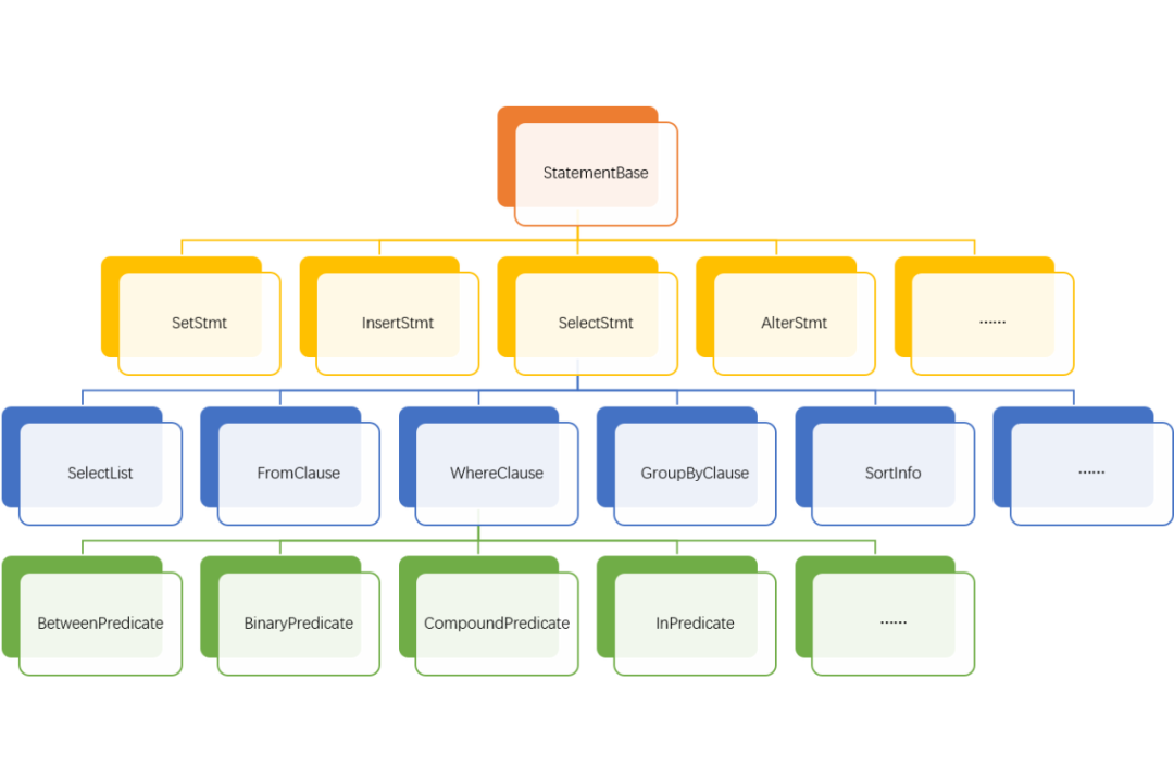
AST has a tree-like structure, which represents a piece of SQL. Therefore, different types of queries -- select, insert, show, set, alter table, create table, etc. will generate additional data structures after Parse (SelectStmt, InsertStmt, ShowStmt, SetStmt, AlterStmt, AlterTableStmt, CreateTableStmt, etc.). However, they all inherit from Statements and will perform some specific processing according to their own grammar rules. For example: for select type SQL, the SelectStmt structure will be generated after Parse.
SelectStmt structure contains SelectList, FromClause, WhereClause, GroupByClause, SortInfo and other structures. These structures contain more basic data structures. For Example, WhereClause contains BetweenPredicate, BinaryPredicate, CompoundPredicate, InPredicate, and so on.
All structures in AST are composed of basic structure expressions--Expr by using various combinations, as shown in Figure 6.
6. Analyze Phase
Analyze will perform pre-processing and semantic analysis on the abstract syntax tree AST generated in the Parse phase, preparing for the generation of stand-alone logic plans.
The abstract class StatementBase represents the abstract syntax tree. This abstract class contains a most crucial member function--analyze(), which is used to perform what's needed to do in Analyze phase.
Different types of queries (select, insert, show, set, alter table, create table, etc.) will generate different data structures through the Parse stage(SelectStmt, InsertStmt, ShowStmt, SetStmt, AlterStmt, AlterTableStmt, CreateTableStmt, etc.), these data structures inherit From StatementBase, and perform a specific Analysis on a specific type sof SQL by implementing the analyze() function.
For example, a query of select type will be converted into analyze() of the sub-statements SelectList, FromClause, GroupByClause, HavingClause, WhereClause, SortInfo, etc. of select SQL. Then these sub-statements further analyze() their sub-structures, and various scenarios of various types of SQL are analyzed by layer-by-layer iteration. For example, WhereClause will further explore the BetweenPredicate, BinaryPredicate, CompoundPredicate, InPredicate, etc., which it contains.
For query type SQL, Analyze will performs several important steps:
-
Metadata identification and parsing: Identify and parse metadata such as Cluster, Database, Table, Column, etc. involved in SQL, and determine which columns, tables, databases, and clusters need to be calculated.
-
SQL correctness check:such as the window function cannot DISTINCT, whether the projection column is ambiguous, the where statement cannot contain grouping operations, etc.
-
Rewrite SQL simply:for example, expand select * to select all columns, convert count distinct to bitmap or hll function, etc.
-
Function correctness check:Check whether the functions contained in SQL are consistent with the system-defined procedures, including parameter types, number of parameters, etc.
-
Aliasing for Table and Column.
-
Type checking and conversion: For example, when the types on both sides of a binary expression are inconsistent, one of the types needs to be converted (with BIGINT and DECIMAL, the BIGINT type needs to be cast to DECIMAL).
After analyzing the AST, a rewrite operation will be performed again to simplify or convert it into a unified processing method. A present rewrite algorithm is a rule-based approach. It will rewrite the AST with each rule from bottom to top, based on the tree structure of the AST. If the AST changes after rewriting, analysis and rewrite will start again until there is no change in the AST.
For example: simplification of constant expressions: 1 + 1 + 1 is rewritten as 3, 1 > 2 is rewritten as Flase, etc. Convert some statements into a unified processing method, such as rewriting where in, where exists as semi join, where not in, where not exists as anti join.
7. Generate stand-alone logical Plan phase
At this stage, algebraic relations will be generated according to the AST abstract syntax tree, also known as the operator number. Each node on the tree is an operator, representing an operation.
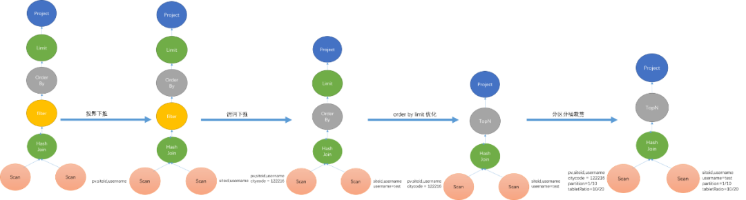
As shown in Figure 7, ScanNode represents scan and read operations on a table. HashJoinNode represents the join operation. A hash table of a small table will be constructed in memory, and the large table will be traversed to find the exact value of the join key. Project means the projection operation, which represents the column that needs to be output at the end. Figure 7 shows that only citycode column will output.
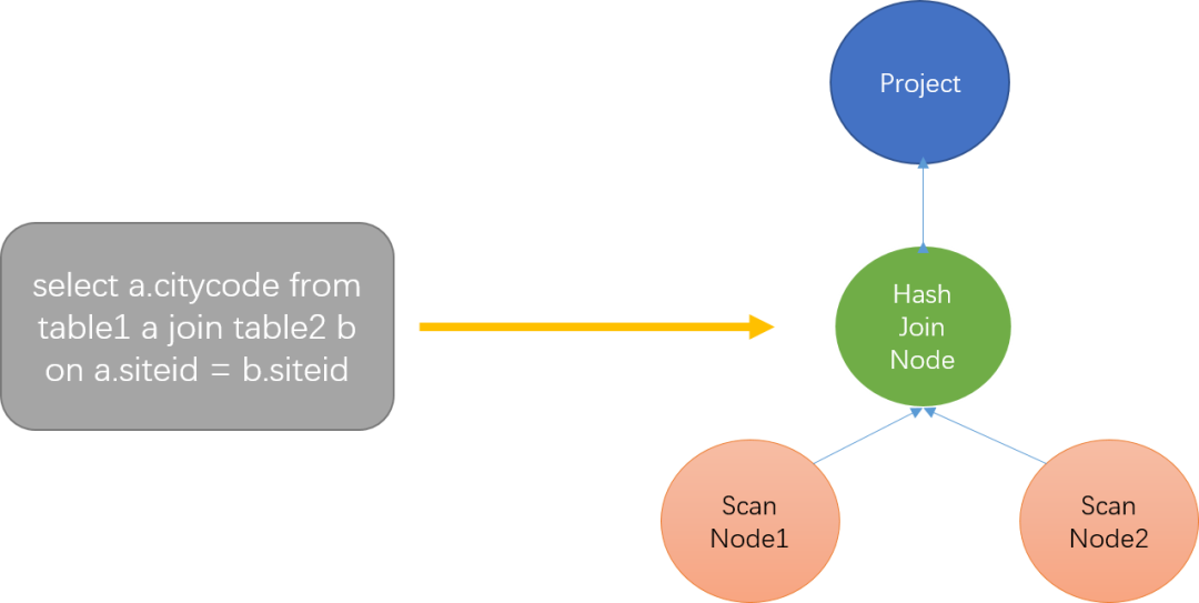
Without optimization, the generated relational algebra is very expensive to send to storage and execute.
For query:
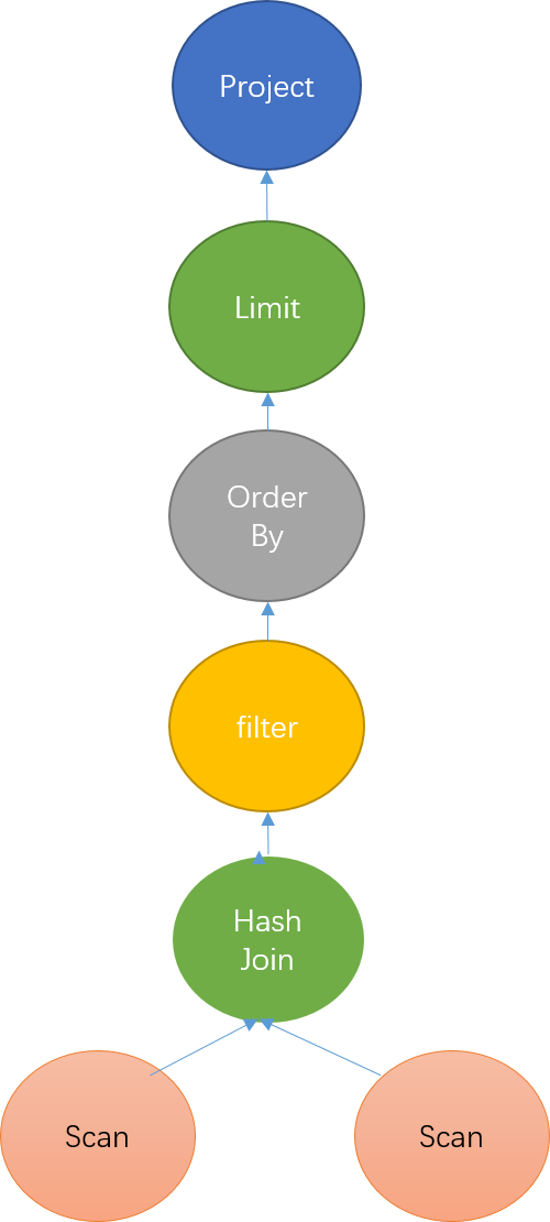
select a.siteid, a.pv from table1 a join table2 b on a.siteid = b.siteid where a.citycode=122216 and b.username="test" order by a.pv limit 10
As shown in Figure 8, for unoptimized relational algebra, all columns need to be read out for a series of calculations. In the end, siteid and pv column are selected and output. A large amount of useless column data wastes computing resources.
When Doris generates algebraic relations, a lot of optimizations are made: the projection columns and query conditions will be put into the scan operation as much as possible.
Specifically, this phase mainly does the following tasks:
-
Slot materialization:Determine the column that needs to be scanned and calculated for the expression. Such as aggregate function expressions and Group By words of aggregate nodes need to be materialized.
-
Projection pushdown:BE only scans the columns that must be read when Scanning.
-
Predicate pushdown:Push down the filter conditions to the Scan node as much as possible under the premise of semantically correct.
-
Partition, bucket cutting:According to the information in the filter conditions, determine which partitions and buckets of tablets need to be scanned.
-
Join Reorder:For Inner Join, Doris will adjust the order of the table according to the number of rows--put the large table in the front.
-
Sort + Limit optimized to TopN:For the order by the limit statement, it will be converted into TopN operation nodes, which is convenient for unified processing.
-
MaterializedView selection: The best-materialized view will be selected according to the columns required by the query, the columns for filtering, sorting and Join, the number of rows, the number of columns, and other factors.
Figure 9 shows an example of optimization. The optimization of Doris is carried out in generating relational algebra. Generating one will optimize one.· Projection pushdown: BE only scans the columns that must be read when Scanning.
8 Generate Distributed Plan Phase
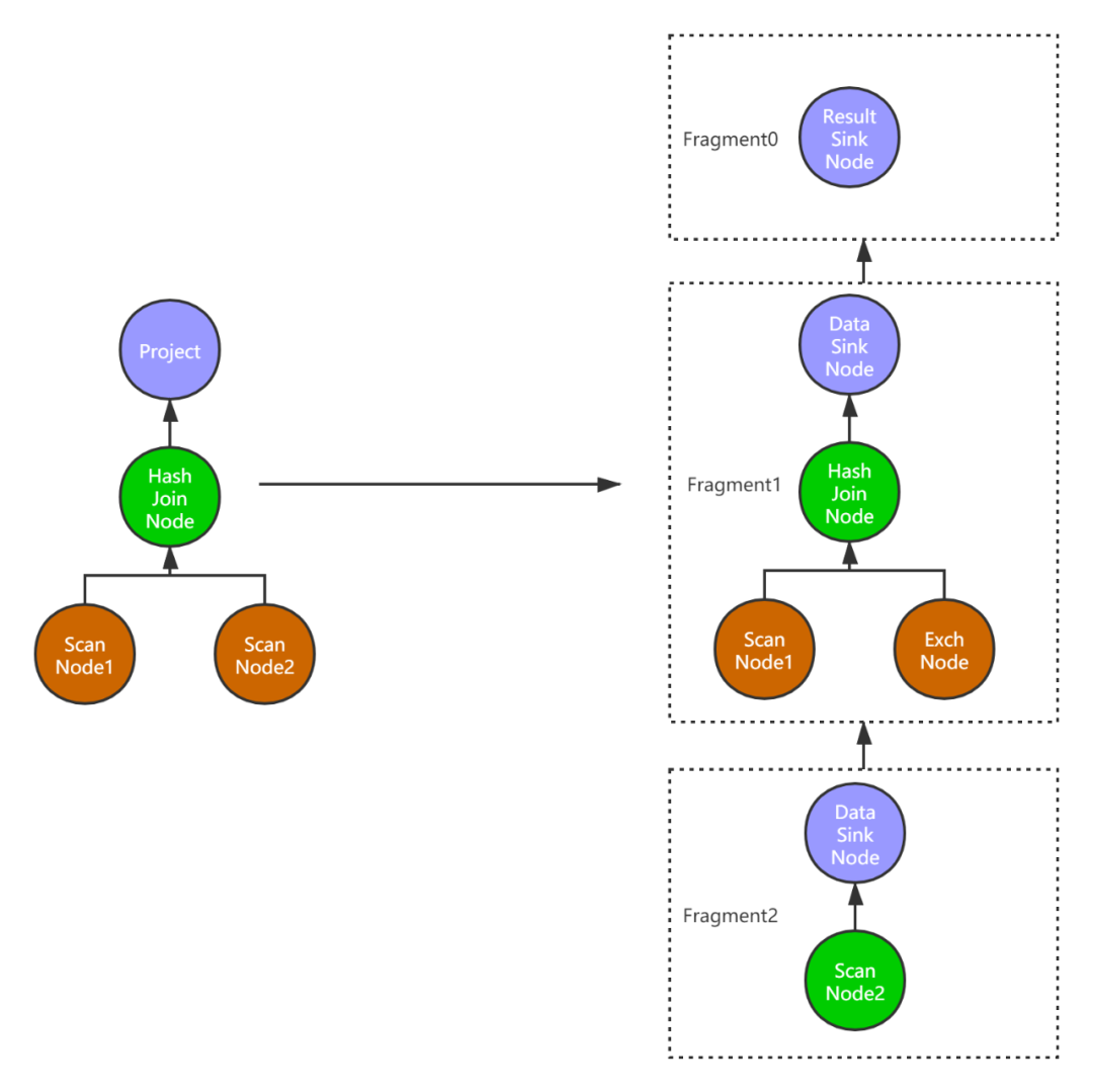
After the single-machine PlanNode tree is generated, it needs to be split into a distributed PlanFragment tree (PlanFragment is used to represent an independent execution unit) according to the distributed environment. A table's data is distributed across multiple hosts could allow some computations to be parallelized.
The primary purpose of this step is to maximize parallelism and data localization. The primary strategy is to split the nodes that can be executed in parallel and create a separate PlanFragment. ExchangeNodes will replace the split nodes to receive data. Finally, a DataSinkNode will be added to the split node to transmit the calculated data to the ExchangeNode for further processing.
This step adopts a recursive method, traverses the entire PlanNode tree from bottom to top, and then creates a PlanFragment for each leaf node on the tree. If the parent node is encountered, splitting the child nodes that can be executed in parallel will be considered.
For query operations, the join operation is the most common.
Doris currently supports four join algorithms: broadcast join, hash partition join, colocate join, and bucket shuffle join.
broadcast join:Send the small table to each machine where the large table is located and perform a hash join operation. When the amount of data scanned from a table is small, the cost of broadcast join will be calculated, and the method with the smallest cost will be selected by calculating and comparing the cost of hash partitions.
hash partition join:When the data scanned from the two tables are both large, hash partition join is generally used. It traverses all the data in the table, calculates the hash value of the key, then modulizes the number of clusters, and whichever machine is selected, the data will be sent to this machine for hash join operation.
colocate join:If the data distribution of the two tables is specified to be consistent when they are created, the colocate join algorithm will be used when the join key of the two tables is the same as the bucket key. Since the data distribution of the two tables is the same, the hash join operation is equivalent to a local process. It does not involve data transmission, which significantly improves query performance.
bucket shuffle join:When the join key is a bucketing key, and only one partition is involved, the bucket shuffle join algorithm is preferred. Since bucketing itself represents a way of dividing data, it only needs to take the hash modulo of the number of buckets from the right table to the left table, so that only one copy of the data in the right table needs to be transmitted over the network, which greatly reduces the network of data transmission, as shown in Figure 10.
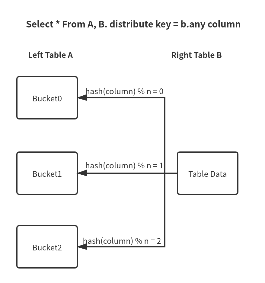
Figure 11 shows the core process of creating a distributed logical plan with a single-machine logical plan with HashJoinNode.
-
For PlanNodes, PlanFragments are created bottom-up.
-
If it is a ScanNode, PlanFragment will be created directly, and the RootPlanNode of the PlanFragment is this ScanNode.
-
If it is a HashJoinNode, the broadcastCost will be calculated at first, which could provide a reference for selecting boracast join or hash partition join.
-
Join algorithm will be chosen according to different conditions.
-
If colocate joins are used, since joins are all local, no splitting is required. Set the left child node of HashJoinNode as the RootPlanNode of leftFragment, and the right child node as the RootPlanNode of rightFragment, share a PlanFragment with leftFragment, and delete rightFragment.
-
If bucket shuffle join is used, data from the right table needs to be sent to the left table. So first create an ExchangeNode, set the left child node of HashJoinNode as the RootPlanNode of leftFragment, the right child node as this ExchangeNode, share a PlanFragment with leftFragment, and specify the destination of rightFragment data to be sent to this ExchangeNode.
-
If broadcast join is used, the data from the right table needs to be sent to the left table. So first create an ExchangeNode, set the left child node of HashJoinNode as the RootPlanNode of leftFragment, the right child node as this ExchangeNode, share a PlanFragment with leftFragment, and specify the destination of rightFragment data to be sent to this ExchangeNode.
-
If hash partition join is used, the data in the left table and the right table must be split, and both left and right nodes need to be split out to create left ExchangeNode and right ExchangeNode respectively. HashJoinNode specifies the left and right nodes as left ExchangeNode and right ExchangeNode. Create a PlanFragment separately and specify RootPlanNode as this HashJoinNode. Finally, specify the data sending destination of leftFragment and rightFragment as left ExchangeNode and right ExchangeNode.
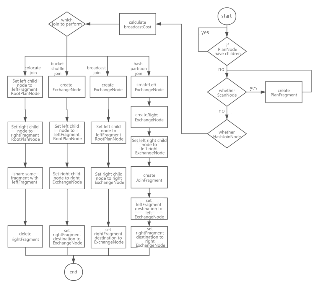
Figure 12 is an example after the join operation of two tables is converted into a PlanFragment tree, there are 3 PlanFragments generated. The final output data passes through the ResultSinkNode node.
9. Schedule phase
This step is to create a distributed physical plan based on the distributed logical plan. will solve the following questions:
-
Which BE executes which PlanFragment
-
Which replica to chooes for each Tablet to query
-
How to perform multi-instance concurrency
Figure 13 shows the core process for creating a distributed physical plan:
a. Prepare phase:Create a FragmentExecParams structure for each PlanFragment to represent all the parameters required for PlanFragment execution; if a PlanFragment contains DataSinkNode, the destination PlanFragment for data transmission will be found, and specify the input of FragmentExecParams of the destination PlanFragment as FragmentExecParams of this PlanFragment.
b. computeScanRangeAssignment phase:Different processing is performed for different types of joins.
-
computeScanRangeAssignmentByColocate: For colocate join processing, since the data distribution in the two table buckets of the join is the same, they are based on the bucket join operation, so here is to determine which host is selected for each bucket. When allocating buckets to hosts, try to ensure that the buckets allocated to each host are even.
-
computeScanRangeAssignmentByBucket: Processing for bucket shuffle join, which is only based on bucket operations, so here is to determine which host is selected for each bucket. When allocating buckets to hosts, it is also necessary to try to ensure that the buckets allocated to each host are even.
-
computeScanRangeAssignmentByScheduler: Process for other types of joins. Determines which replica of the tablet each scanNode reads. A scanNode will read multiple tablets, and each tablet has various copies. To distribute the scan operation on various machines as much as possible, improve concurrent performance, and reduce IO pressure, Doris uses the Round-Robin algorithm to distribute tablet scans to multiple machines as much as possible. For example, 100 tablets need to be scanned, each tablet has three copies, and ten machines could be used. When allocating, each machine is guaranteed to scan ten tablets.
c.computeFragmentExecParams phase:This stage determines which BE the PlanFragment is issued to for execution and how to handle instance concurrency. After the scan address of each tablet is determined, FragmentExecParams will generate multiple instances with the address as the dimension. If various addresses are contained in FragmentExecParams, various instances of FInstanceExecParam will be generated. If the concurrency is set, the execution instance of an address will be further split into multiple FInstanceExecParams. There will be some special processing for bucket shuffle join and colocate join, but the basic logic is the same. After FInstanceExecParam is created, a unique ID will be assigned to facilitate tracking information. If FragmentExecParams contains ExchangeNode, the number of senders will be counted to know how many senders' data needs to be accepted. Finally, FragmentExecParams determines the destinations and fills in the destination address.
d. Create result receiver stage:The resulting receiver is where the final data needs to be output after the query is completed.
e. to thrift stage:Create RPC requests based on FInstanceExecParam of all PlanFragments, then send them to the BE side for execution. A complete SQL parsing process is completed.
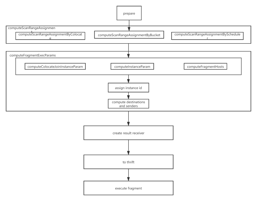
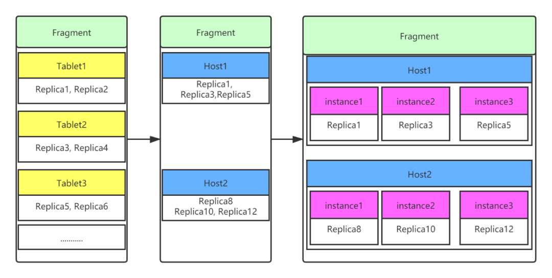
Figure 14 is a simple example. The PlanFrament in the figure contains a ScanNode. The ScanNode scans three tablets. Each tablet has two copies, and the cluster assumes that there are two hosts.
The computeScanRangeAssignment stage determines that replicas 1, 3, 5, 8, 10, and 12 need to be scanned, where replicas 1, 3, and 5 are located on host1, and replicas 8, 10, and 12 are located on host2.
If the global concurrency is set to 1, 2 instances of FInstanceExecParam are created and sent to host1 and host2 for execution. If the global concurrency is set to 3, 3 instances of FInstanceExecParam are created on this host1, and three instances of FInstanceExecParam are created on host2. Each instance scans one replica, equivalent to initiating 6 RPC requests.
10 Summary
This article first briefly introduces Doris and then introduces the general process of SQL parsing: lexical analysis, syntax analysis, generating logical plans, and generating physical plans. Then, it presents the overall architecture of DorisSQL parsing. In the end, the five processes: Parse, Analyze, SinglePlan, DistributedPlan, and Schedule are explained in detail, and an in-depth explanation is given of the algorithm principle and code implementation.
Doris complies with the standard methods of SQL parsing. Still, according to the underlying storage architecture and distributed characteristics, many optimizations have been made in SQL parsing to achieve maximum parallelism and minimize network transmission, reducing a lot of burden on the SQL execution level.